

Two types of rainfall data are generally needed when dealing with natural hazards. Longer time series with daily data that can be used for a frequency magnitude analysis, while detailed intensity data are needed for flood modelling and engineering (hydraulic) design purposes. Of the 4 islands in CHARIM Saint Lucia has by far the most complete network of stations, with 18 stations that have daily totals since 1954 and 8 more recent stations that give minute rainfall intensities. There are more stations on the island but their records are more erratic and not used in this analysis. Of the other islands only 2 -4 stations with daily totals. These record are often measured at the national airports or capitals of the islands.
Keywords:
rainfall, frequency analysis, Saint Lucia, intensity-duration, gumbel, GEV
| Before you start: | Use case Location: | Uses GIS data: | Authors: |
|---|---|---|---|
| Read session 2.3 of the Methodology book for more information | This use case uses data from Saint Lucia | No | Victor Jetten, Jovani Yifru and Cees van Westen |
Objectives:
Analyze the long term records of daily rainfall data of each island to determine the rainfall depth for 5, 20, 20 and 50 years (the return periods used in the flood analysis). A probability density analysis for the return periods of annual daily maxima is used. If more than one station exists, average values are used based on expert judgement.
Create design rainfall events for each of the return periods with 5 minute interval data. These can be used for flood hazard modeling and engineering design.
Data requirements:
There are 18 stations on St Lucia that have long records, mostly from 1955 to 2014. The location of the stations is shown in figure 1. Not all stations have full records for the entire period (varying from 21 to 54 years with daily data, see Figure 2 for an impression of the quality of the stations). Years with less than 60% of the days with valid records were excluded. Many of the stations have been upgraded to full automatic stations from 2003 onward with measurements at 1 minute resolution. However of these stations, 2005-2008 were frequently missing and there are spurious values (intensities impossible with respect to the maximum a tipping bucket can record which usually lies around 270 mm/h).
Figure 1: Rainfall stations on St Lucia. Left: stations represented as yellow dots are used in the frequency magnitude analysis (1955-2005). Right: average annual rainfall (Marmagne and Fabrègue, 2013)
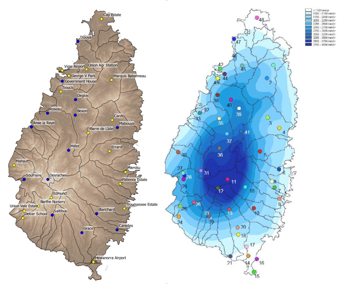
Figure 2: An impression of the Station record quality, with 0% = missing data. The 18 stations are given in Figure 1 as yellow dots.

A hand check for spurious values is needed: if an extreme event occurs for one station, but not for any of the others it is excluded. However, not all stations always record an event on the same day, sometimes a value is the sum of several days, see figure 3. This is an example of Hurricane Debbie (9/9/1994). It shows that for some records, the instrument has not been read for a number of days, and the rainfall is therefore an accumulated reading (stations Cap and Hewanorra). It was therefore assumed that the maximum recorded daily rainfall in a 10 day period is from the same storm event.
Figure 3: Example of station recordings for hurricane Debbie on 9 Sep 94. Arrows show likely delayed reading.

Analysis steps:
Return period:
- Clean the daily records by eliminating extreme and spurious values, and eliminate years with more than 40% of the days having missing values.
- For each station, identify the daily maximum value for each year and retain the date of occurrence
- Analyze the distribution of extreme values with a Gumbel analysis and a GEV analysis (General Extreme Value distribution).
- Determine the daily totals for 5, 10, 20 and 50 year recurrence intervals.
- Repeat step 1 to 4 for each island.
Design storms:
- Isolate all events from the tipping bucket data of the Saint Lucia stations, with storm depths in the same order of magnitude as the 5 to 50 year daily totals
- Fit a probability density function to these events, looking at intensity, depth and duration
Results:
Daily maxima recurrence intervals
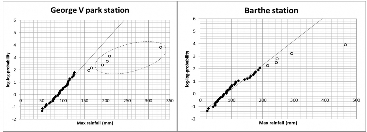
Initially Gumbel distributions were fitted to each station. A Gumbel distribution is a special case of Generalized Extreme Value distributions, suitable for right hand skewed datasets (such as rainfall, that cannot be less than 0, but can have extreme maxima). The Gumbel distribution assumes a double logarithmic relation between the maximum rainfall R and the return period T. The return period is the inverse of the probability P. As an example, Figure 4.4 shows the Gumbel analysis of George V Park in Castries. The station is close to Bois d’Orange river and Choc river north of Castries (St Lucia), that are both known to flood occasionally. It can be seen that a Gumbel analysis linearizes a part of the data, but the 6 highest values are not on the same line. When searching for the dates corresponding to these days, it appears that the 4 largest at least are known class 5 hurricanes (NOAA Hurricane Database, http://www.nhc.noaa.gov/).
Figure 4: Example Gumbel analysis of maximum daily values of Barthe station and George V park station (1955-2005). The four encircled highest values for George V park correspond from low to high to category 5 hurricanes: Aug-Sep 1960 - Donna; Aug-Sep 1980 - Allen; Sep 1988 - Gilbert and Sep 1967 - Buela. For Barthe the highest values correspond with: Oct 1970 - Tropical depression 19, hurricanes Buela and Gilbert and May 1987 tropical depression 1
Two conclusions are drawn from this:
- The Gumbel analysis does not succeed in fitting the entire dataset of each station, the data is too skewed.
- The hurricane data is not enough for a separate statistical analysis, as there are "only" 4-6 years per station with hurricanes and tropical storms.
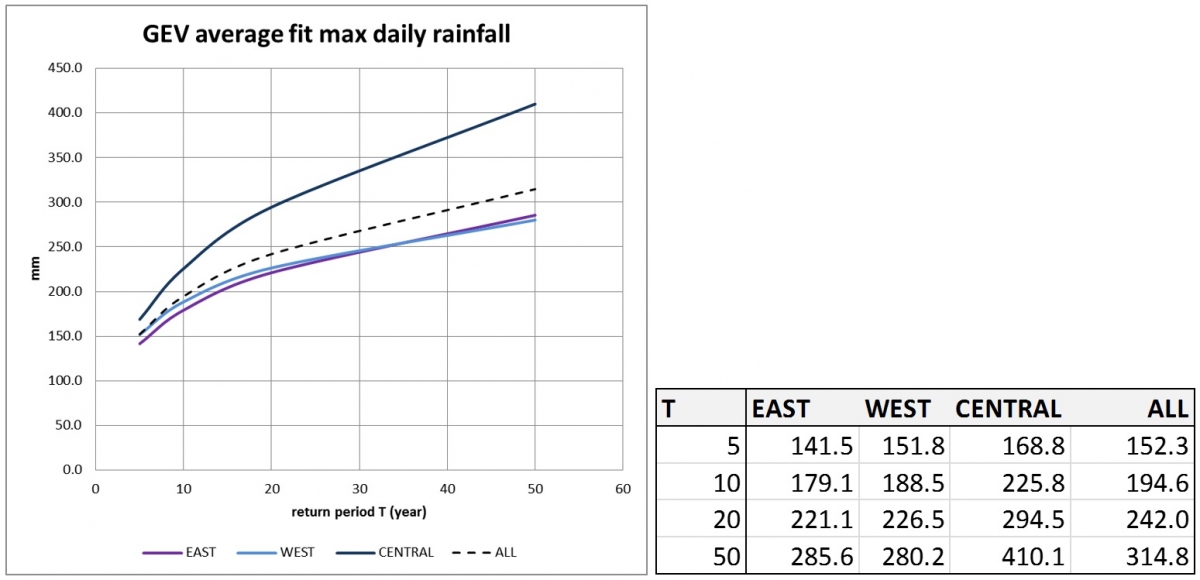
It was decided to abandon Gumbel and use a Generalized Extreme Value (GEV) distribution fit. The equation has more parameters that allow for a better linearization of the data (see e.g. Coles, 2001). Each station was fitted with a GEV distribution. The parameters of the distribution are given in Figure 9. The stations are grouped with respect to their location on the island: the neat coastal stations in the east (E), the near coastal stations in the west (W) and the stations further from the coast towards the center of the island (C). This grouping was done to explore if there are differences relative to the position of the station. According to Klein Tank et al. (2009), mu and sigma are location parameters that are surprisingly stationary and can be averaged for different stations, while k is a shape parameter that has a more local nature. Figure 10 shows the curves using the averages of the fit parameters k, mu and sigma: it can be seen that the east and west of the island show very little difference in return periods structure, while the center of the island has much higher daily maxima for the same return period values.
It was decided to simply use the average of the fitting parameters of all stations. Because there are 12 coastal zone stations and 5 inland stations in the dataset, this gives a weighted average, i.a. the coastal zone stations dominate. This was considered acceptable as most inhabitation is in the coastal zone.
Figure 5: Left: GEV distribution fit parameters for 19 stations. The indication E, W and C corresponds to stations near the east coast, near the west coast and closer to the center of the island. Right: GEV equations

Figure 6: Left: GEV analysis of stations in fig 4.5. The coastal zone stations for the east and west side of the island are not significantly different. Right resulting near coastal GEV return periods and daily maxima. Right: the corresponding return period T and average daily maximum values used in the hazard analysis
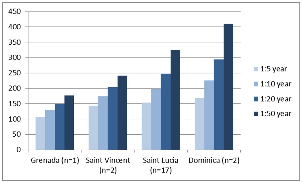
Looking at the GEV analysis of the other islands in CHARIM (Grenada, St Vincent and the Grenadines, and Dominica), a north south gradient can be clearly seen in the design storm depth based on the GEV analysis of daily maxima. A possible explanation lies in the nature of hurricanes and severe tropical storms, they cross the Atlantic at the equator and veer north due to Coriolis forces. They influence local weather systems as well, which possibly leads to a North-South gradient in amount of rainfall in the Caribbean. However it should be noted that apart from Saint Lucia, the other islands have only 1 or 2 stations with long records, normally near the airport or the capital. A north-south trend should be seen as a possible indication at best.
Figure 7: Return periods and daily maxima from GEV analyses of rainfall stations at the 4 islands in CHARIM. While the islands are analyzed independently, a general trend can be seen from north to South
Design storms
A hazard analysis cannot be done on actual rainfall events because this would make the comparison between events of different magnitude impossible, if they are spatially very different. Design rainfall event have to be used. Design storms are used mostly in civil and construction engineering to calculate proper dimensions of channels, culverts and bridges. These are events that correspond to a certain shape, size and duration for each return period that is needed (in this case 5, 10, 20 and 50 years). The total size of the design events (the rainfall depths) should be identical to the GEV analysis sizes in Figure 7.
A common way to create a design event is from intensity-duration-frequency curves, or IDF curves. A few such curves exit for the region, but mainly for the northern part of the Caribbean. Lumbroso et al. (2011) constructed IDF curves for the Bahamas (Figure 8). IDF curves also exist for the Florida but those are considered not representative as they are too far north and the climate might be dominated by the US landmass.
Figure 8: IDF curves for the Bahamas (Lumbroso et al., 2011)
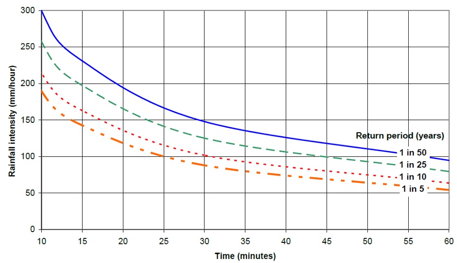
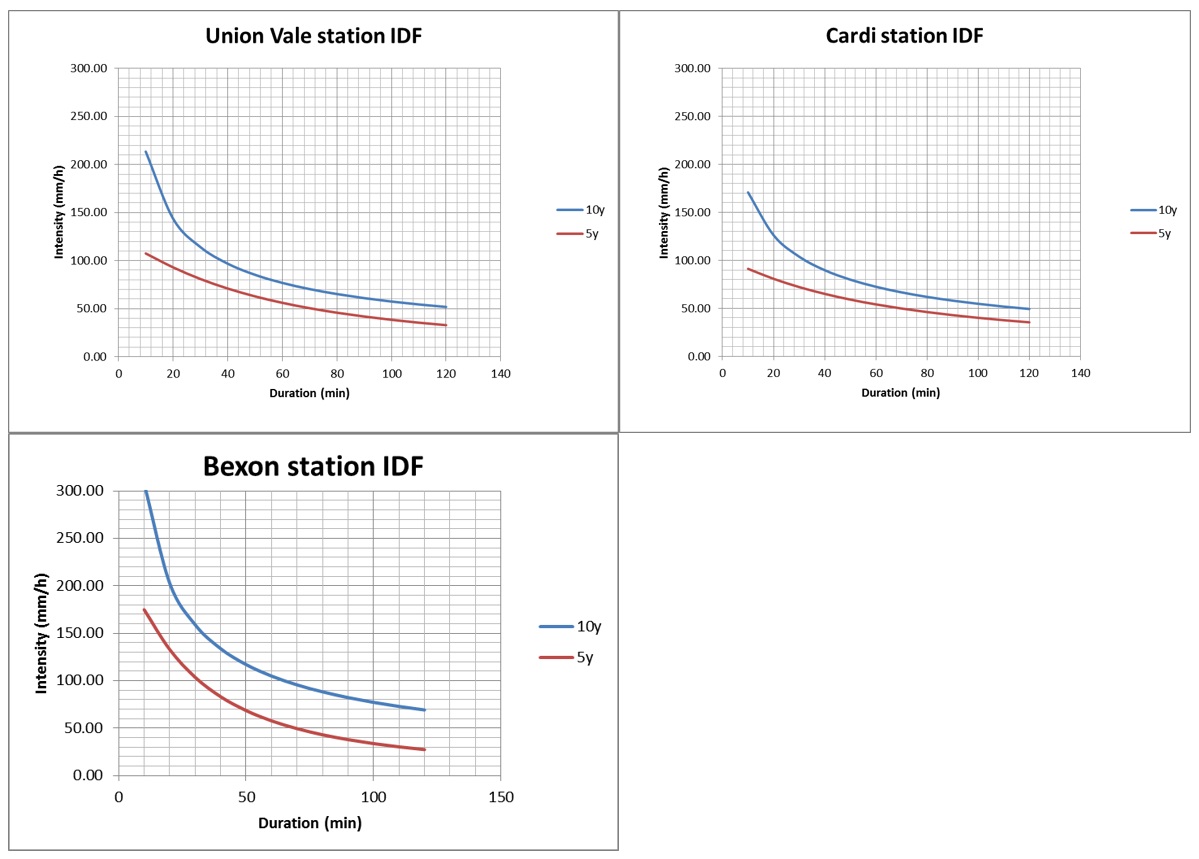
Of the Saint Lucia high resolution weather stations that are operational since 2005, 3 had a consistent continuous rainfall record that enabled the construction of IDF curves, for 5 and 10 years (Figure 9). Curves for longer return periods cannot be created because the series are not large enough. It can be seen that Bexon station has higher rainfall intensities. This could be because of its elevation, but Cardi is in a similar position and has much lower intensities. Bexon station curves resemble the Bahamas curves of Lumbroso et al. (2011), but the difference between 5 and 10 year is more pronounced for the higher intensities.
Figure 9: IDF curves for 3 stations that have 10 years of intensity data
From IDF curve design storms can be created using the alternating block method (Chow et al., 1988). The design storms are shown in Figure 10. Unfortunately, the rainfall derived from the IDF curves do not have the correct depth compared to the GEV analysis (the rainfall events are all approximately 50% smaller). A possible explanation is the short time series that is at the basis of this analysis, within 10 years the range of intensities that are captured by the 3 stations does not resemble the intensities of the larger dataset of the 17 stations of the GEV analysis.
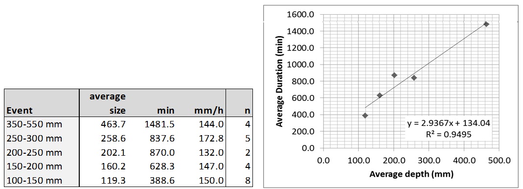
We therefore decided not to use the IDF data but analyze the rainfall events directly. In total 35 rainfall events existed of 90 mm and larger, based on the 1 minute intensity data of 15 stations over a period of 3 to 10 years (depending on the station). These events were grouped according to total depths. Of course the larger events only have a few realizations, a summary is given in Figure 15. Average depth and duration are well correlated, while the average maximum intensity does not show any correlation with event size. In other words, larger rainfall events are longer in duration, but not necessarily more intense. In reality they are very complex with temporal and spatial variability.
Figure 10: Design storms for 5 and 10 years for 3 stations that have 10 years of data. The events are created with the alternating block method from the IDF curves
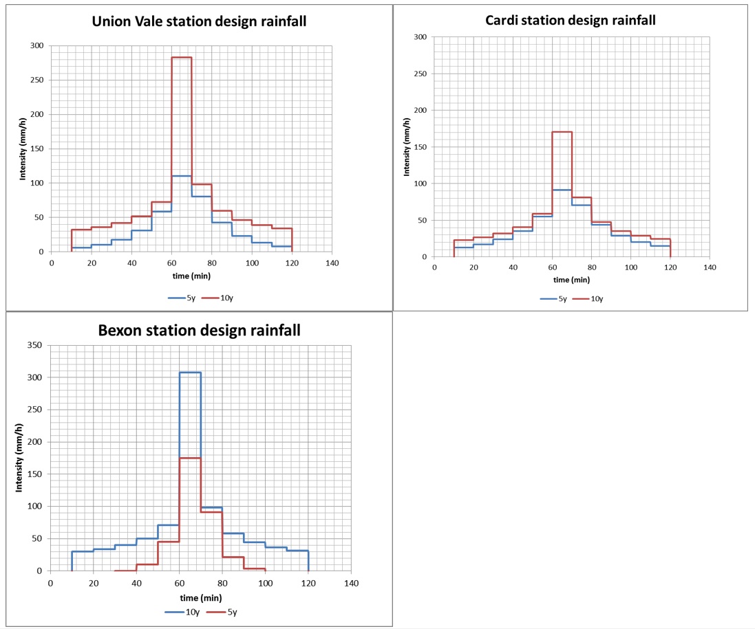
Figure 11: Summary characteristics of the 23 largest events, from 15 stations in 10 years. Average depth and duration are well correlated, while the average maximum intensity does not show any correlation with event size
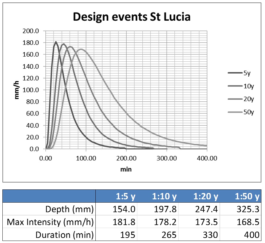
Within each class the events were fitted with probability density function, for which a Johnson SB distribution was used. This distribution gave the best results. This resulted in the a set of Johnson SB distribution parameters for each class. These were then scaled up so that the curve describing the rainfall event has a depth and intensity close to the measured average maximum intensities. This resulted in the design events shown in fig 8.12. There is a gradual decrease in peak intensity form 5 to 50 years return period, and a larger storm depth. The duration of the design storms is considerably shorter than the real average duration as shown in Figure 8.11, which is because in the real events there are frequently short periods with low amounts of rainfall while the design events is a single closed event.
Figure 12: Design storms for St Lucia for 4 return periods, based on a Johnson SB distribution fit to representative rainfall events in the classes shown in figure 11
Conclusions:
Frequency magnitude analysis of rainfall is best done with a GEV (General Extreme value) distribution, as it succeeds better in capturing the extreme events such a Hurricanes, in a single distribution. Nevertheless class 5 hurricanes and tropical storms seem to be a separate class, that are not part of the regular statistical distribution. It is not known why and data is too scarce to analyze this. The Saint Lucia network is one of the best in the Caribbean, offering sufficient data for a GEV analysis. It can be seen that there is little difference between the Atlantic and the continental side in terms of rainfall, but there central (higher elevated) part of the island has a different frequency magnitude distribution. This is also known from the annual total rainfall distribution.
Design events used for modelling and engineering can be constructed with a Johnson SB distribution of selected measured events, but the datasets are too short for a thorough IDF curve analysis and subsequent design storm construction. The data of only 3 stations is just sufficient for a 5 and 10 year IDF curve, but the period is very short and likely does not capture the full range of intensities.
References:
Chow, V.T., Maidment, D.R. and Mays, L.W. 1988. Applied Hydrology. McGraw-Hill Publishing Company; International edition. pp588.
Klein Tank, A.M.G., Zwiers, F.W. and Xuebin Zhang. 2009. Guidelines on Analysis of extremes in a changing climate in support of informed decisions for adaptation. WMO Climate Data and Monitoring WCDMP-No. 72.
Lumbroso, D.M., S. Boyce, H. Bast and N.Walmsley. 2011. The challenges of developing rainfall intensity – duration – frequency curves and national flood hazard maps for the Caribbean.
Last update: 06 - 04 - 2016