

This section introduces the concept of magnitude frequency analysis and gives examples of the generation of magnitude-frequency relations for flooding and landslides.
Keywords: magnitude, frequency, flooding, landslides.
Authors: Cees van Westen, Victor Jetten
Links:
- Use case 8.2 on magnitude-frequency analysis.
- Collection of historical data
- Collection of Hydro-Met data
- Flood susceptibility assessment
Introduction
As described in section 2.1, the most important aspects of hazards are the spatial and temporal characteristics of the events. One of the most important temporal characteristic of a hazardous event is the frequency of occurrence. Frequency is:
- the rate of occurrence of a phenomena;
- the relationship between incidence and time period;
- the number of occurrences within a certain period of time;
- the quotient of the number of times n a periodic phenomenon occurs over the time t in which it occurs: f = n / t
- the (temporal) probability that a hazardous event with a given magnitude occurs in a certain area in a given period of time (years, decades, centuries etc.).
In hazard assessment, frequency is a key point to study the occurrence probability of hazardous events in the future. The analysis of historical records and their frequency allows scientists to understand when a certain hazard with a certain magnitude is likely to occur in a given area. In most of the cases there is a fixed relation between magnitude and frequency for natural events (see figure 1). The frequency of events with a low magnitude is high, while the frequency of events with great magnitude is low: i.e. small flood events occur every year while enormous and devastating inundations are likely to happen once every one or more centuries. Magnitude-frequency relationship is a relationship where events with a smaller magnitude happen more often than events with large magnitudes. For rainfall phenomena both small magnitudes as well as large magnitudes may be catastrophic as illustrated in figure 1.
Figure 1: Graphs showing the magnitude - frequency relation for rainfall related events.
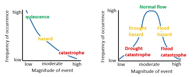
Few hazards don't follow this rule; an example of events with random relation between magnitude and frequency is lightning. Frequency is generally expressed in terms of exceedance probability; which is defined as the chance that during the year an event with a certain magnitude is likely to occur. The exceedance probability can be shown as a percentage: a hazard, that statistically occurred once every 25 years, has an exceedance probability equal to 0.25 (or 25%). Another method is the calculation of the return period: it indicates the period in years in which the hazards is likely to occur based on historic records; an example can be a flood with a return period of 100 years (100 years return period flood = 1 event in 100 years = 0.01 probability).
Figure 2: Relation between magnitude and frequency. Hazard A shows a relationship where the same magnitude may occur much more frequent than for hazard B.
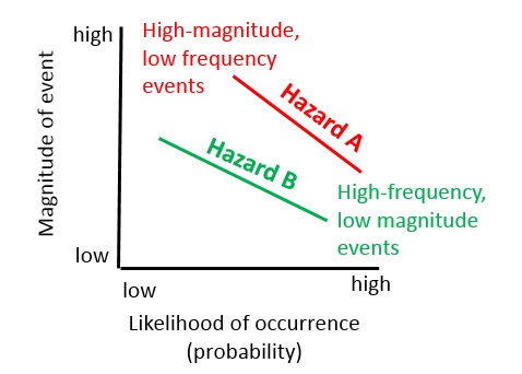
Most hazard types display a relationship between the likelihood of occurrence (probability) and the magnitude of the event, as shown in figure 2. This relationship might differ substantially depending on the hazard type. The frequency magnitude relationship can be valid for the same location (e.g. a particular slope, x-y location, building site). This is the case for events like flooding, where each location will have its own height-frequency relationship depending on the local situation. The flood itself will also have its own discharge-frequency relationship for the entire catchment, but this can be used as input to calculate the height-frequency relationship for a particular point. In other cases the frequency magnitude relationship cannot be established for an individual point, but is done for a larger area (e.g. catchment, province, country, globe). For instance the occurrence of landslides cannot be represented for a particular location as a magnitude-frequency relationship (except for debris flows and rock fall) as the occurrence of a landslide will modify the terrain completely. Thus you cannot say that small landslides occur often in the same location and large landslide less frequently. However, you can say that for an entire watershed.
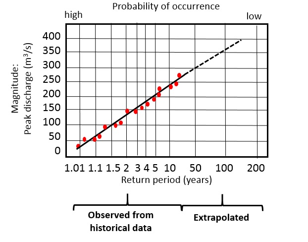
A frequency-magnitude relationship is normally based on a historical record of hazardous events (See previous section 2.2). This is illustrated in Figure 3, where data is available for a 25 year period. The maximum discharge measured per year is plotted after it was ordered from high to low, and the regression line shows the magnitude-frequency relation for these observed data. For larger return periods there are no observed data anymore and therefore the regression line is extrapolated. Obviously, the shorter the observed period is, the less reliable will be the regression line, and the higher will be the uncertainty of the extrapolated line.
Figure 3: Frequency magnitude example for flooding, showing the relation between flood discharge, return period and probability.
Historical information is always incomplete, as we can only obtain information over a particular period of time, e.g. the period over which there was a network of seismographs. The length of the historical record is of large importance for accurately estimating the magnitude-frequency relation. If the time period is too short, and didn't contain any major events, it will be difficult to estimate the probability of events with large return periods. The accuracy of prediction also depends on the completeness of the catalog over a given time period. In the case that many events are missing, it will be difficult to make a good estimation.
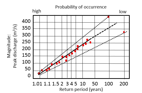
Also when the measurement period contains a large outlier (an event with a much higher magnitude than the others) the results may also be ambiguous. This is illustrated in figure 4, showing the range of uncertainty due to the occurrence of two events with higher magnitude.
Figure 4: Uncertainty in magnitude-frequency relation due to the occurrence of outliers.
In the following section examples are given of the generation of magnitude-frequency relations: for flooding, and landslides.
Flood frequency analysis
Hydrologic systems are sometimes impacted by extreme events, such as severe storms, floods, and droughts. The magnitude of such an event is inversely related to its frequency of occurrence, very severe events occurring less frequently than more moderate events. The objective of frequency analysis of hydrologic data is to relate the magnitude of extreme events to their frequency of occurrence through the use of probability distributions. The hydrologic data analysed are assumed to be independent and identically distributed, and the hydrologic system producing them (e.g. a storm rainfall system) is considered to be stochastic, space-independent, and time-independent.
Table 1: Example of maximum discharge values measured in a watershed in the period 1965 - 2008. Values higher than 50000 are indicated in bold.
|
Year |
1960 |
1970 |
1980 |
1990 |
2000 |
|---|---|---|---|---|---|
0 1 2 3 4 5 6 7 8 9 |
38500 179000 17200 25400 4940 |
55900 58000 56000 7710 12300 22000 17900 46000 6970 20600 |
13300 12300 28400 11600 8560 4950 1730 25300 58300 10100 |
23700 55800 10800 4100 5720 15000 9790 70000 44300 15200 |
9190 9740 58500 33100 25200 30200 14100 54500 12700 |
The hydrologic data employed should be carefully selected so that the assumptions of independence and identical distribution are satisfied. In practice, this is often achieved by selecting the annual maximum of the variable being analysed (e.g. the annual maximum discharge, which is the largest instantaneous peak flow occurring at any time during the year) with the expectation that successive observations of this variable from year to year will be independent.
The results of flood flow frequency analysis can be used for many engineering purposes: for the design of dams, bridges, culverts, and flood control structures; to determine the economic value of flood control projects; and to delineate flood plains and determine the effect of encroachments on the flood plain.
Return period
Suppose that an extreme event is defined to have occurred if a random variable X is greater than or equal to some level xT. The recurrence interval t is the time between occurrences of X >= xT. For example, table 1 shows the record of annual maximum discharges of a river, from 1965 to 2008. If xT = 50000 m3/s, it can be seen that the maximum discharge exceeded this level nine times during the period of record, with recurrence intervals ranging from 1 year to 16 years, as shown in table 2
Table 2: Years with annual maximum discharge equalling or exceeding 50000 m3/s and the corresponding recurrence intervals
|
Years were 50000 is exceeded |
1966 |
1970 |
1971 |
1972 |
1988 |
1991 |
1997 |
2002 |
2007 |
Average |
|---|---|---|---|---|---|---|---|---|---|---|
|
Recurrence interval |
|
4 |
1 |
1 |
16 |
3 |
6 |
5 |
5 |
5.1 |
The return period T of the event X >= xT is the expected value of t, E(t), its average value measured over a very large number of occurrences. For the data, there are 8 recurrence intervals covering a total period of 41 years between the first and last exceedance of 50000 m3/s, so the return period of a 50000 m3/s annual maximum discharge is approximately T = 41/8 = 5.1 years. Thus the return period of an event of a given magnitude may be defined as the average recurrence interval between events equal or exceeding a specified magnitude.
The probability p = P(X >= xT) of occurrence of the event X >= xT in any observation may be related to the return period in the following way. For each observation, there are two possible outcomes: either "success" X >= xT (probability p) or "failure" X < xT (probability 1-p). Since the observations are independent, the probability of a recurrence interval of duration T is the product of the probabilities of t-1 failures followed by one success, that is, (1- p)t-1.p.
Assuming that the series of data is infinite, the E(T) can be expressed as:
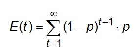 Eq 1
Eq 1
Developing this expression in terms and after some algebra:
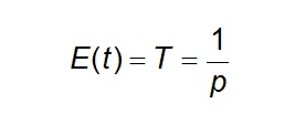 Eq 2
Eq 2
Therefore, the probability of occurrence of an event in any observation is the inverse of its return period.
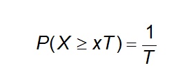 Eq 3
Eq 3
For example, the probability that the maximum discharge will equal or exceed 50000 m3/s in any year is approximately p= 1/t= 1/5.1= 0.195 (19.5%)
Suppose a certain flood (F) has a probability of occurrence of 10% - meaning a probability of 10% that this flood level will be reached or exceeded.
In the long run, the level would be reached on the average once in 10 years. Thus the average return period T in years is defined as:
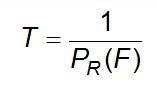 Eq 4
Eq 4
and the following general relations hold:
The probability that F will occur in any year:
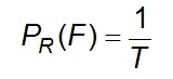 Eq 5
Eq 5
The probability that F will not occur in any year
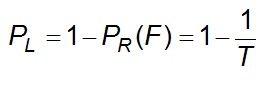 Eq 6
Eq 6
The probability that F will not occur in any of n successive years
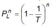 Eq 7
Eq 7
The probability R, called risk, that F will occur at least once in n successive years
 Eq 8
Eq 8
Extreme value distributions
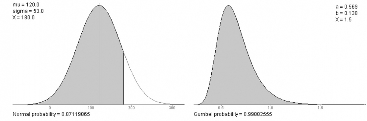
A large amount of process events in hydrology are right skewed, leading to differences between the mode, median and mean of their distributions (see figure 5).
Figure 5: Left: A normal distribution accurately describes facts in nature that apart evenly for a mean. Right: River discharges and rainfall are right skewed events. Their value cannot be lower than zero and extreme events might occur far from the average.
There are a number of influences that promote this characteristic right-skewness of recorded natural events:
- Where the magnitude of given events is absolutely limited at the lower end (i.e. it is not possible to have less than zero rainfall or runoff), or is effectively so (i.e. as with low temperature conditions), and not at the upper end. The infrequent events of high magnitude cause the characteristic right skew.
- The above-mentioned limitation of the lower magnitudes implies that as the mean of the distributions approaches this lower limit, the distribution becomes more skewed.
- The longer the period of record, the greater the probability of observing infrequent events of high magnitude, and consequently the greater the skewness.
- The shorter the time interval within measurements are made, the greater the probability of recording infrequent events of high magnitude and the smaller the skewness.
- Other physical principles tend to produce skewed frequency distributions. For example the limited size of high intensity thunderstorms means that the smaller the drainage basin, the higher the probability that it will be completely blanked by heavy rain and this leads to an increase in skewness in the distribution of runoff as basin size decreases. Similarly, stream discharge frequencies are extremely skewed where impermeable strata allow little infiltration.
The right skewed distributions present certain problems of description and of inferring probabilities from them. When plotted on linear-normal probability paper, right skewed distributions appear as concave curves.
There are three methods to calculate the extreme value distribution in case of right skewness: Gumbel, Frechet and Weibull, see Fig 6. These methods are called the Extreme Value methods (EV's) and they are all based on one general equation called the General Extreme Value (GEV) distribution. The extreme value transformation or double exponential transform is extensively used to straighten out cumulative plots of highly skewed distributions. The Generalized Extreme Value (GEV) distribution is a flexible three-parameter model that combines the Gumbel, Frechet, and Weibull maximum extreme value distributions.
Figure 6: Gumbel, Frechet and Weibull extreme value distributions and the Generalized Extreme Value distribution.
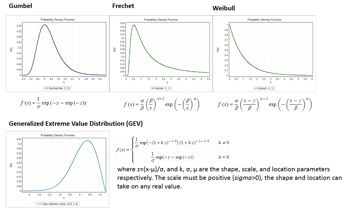
The Gumbel distribution is a distribution with a light upper tail and it is positively skewed. It often underestimates the actual situation. Frechet gives a better estimation, but as three variables are needed for Frechet and just two for Gumbel, the Gumbel method is generally used. Frechet is a distribution with a heavy upper tail and infinite higher order moments. The Weibull distribution is a distribution with a bounded upper tail. It used to estimate the drought. For this method, also three variables are needed.
Critical notes extreme frequency analysis
It is important to realize what exactly a return period (or recurrence interval) of 1:X years actually means. A 1:5 year storm means that on average over a long period, a storm of a given magnitude and duration is exceeded once every 5 years. This does not mean that a 5-year storm will happen regularly every 5 years, or only once in 5 years, despite the connotations of the name "return period". In any given 5-year period, a 5-year event may occur once, twice, more, or not at all.
This can be explained as follows. Statistically the probability of a 1:5 year storm occurring is 0.2 per year, and therefore each year it has a probability of 0.8 of not occurring. If the storm hasn't happened several years in a row, the probability that it will occur in the following year increases. If it hasn't happened in 2 years, the probability of not occurring is reduced to 0.8*0.8=0.64. If it hasn't happened 5 years in a row, the probability of the storm not occurring has reduced to 0.85 = 0.33, and so forth. The probability that it will occur after 5 years of not occurring is 1-0.33 = 0.67. In other words, there is a 67% chance that a 1:5 year storm occurs after the next 5 years. Continuing this reasoning it is 99% certain that such a storm will happen within the next 20 years.
The statistical methods discussed are applied to extend the available data and hence predict the likely frequency of occurrence of natural events. Given adequate records, statistical methods will show that floods of certain magnitudes may, on average, be expected annually, every 10 years, every 100 years and so on. It is important to realize that these extensions are only as valid as the data used. It may be queried whether any method of extrapolation to 100 years is worth a great deal when it is based on (say) 30 years of records. Still more does this apply to the '1000 year flood' and similar estimates. As a general rule, frequency analysis should be avoided when working with records shorter than 10 years and in estimating frequencies of expected hydrologic events greater than twice the record length.
Another point for emphasis is the non-cyclical natural of random events. The 100-year flood (that is, the flood that will occur on average, once in 100 years) may occur next year, or not for 200 years or may be exceeded several times in the next 100 years. The accuracy of estimation of the value of the (say) 100-year flood depends on how long the record is and, for floods, one is fortunate to have records longer than 30 years. Notwithstanding these warnings, frequency analysis can be of great value in the interpretation and assessment of events such as flood and the risks of their occurrence in specific time periods.
Additional Resources:
- EasyFit: EasyFit allows to automatically or manually fit a large number of distributions to your data and select the best model in seconds. It can be used as a stand-alone application or with Microsoft Excel, enabling you to solve a wide range of business problems with only a basic knowledge of statistics.
- RStudio. RStudio has an extreme value analysis package called "extRemes" (Gilleland, 2015). Two functions contained in this package were used for the analysis namely: Fit an Extreme Value Distribution to Data (FEVD) and Likelihood-Ratio Test (LR.test). The FEVD function can be used to fit the data into GEV distribution model or Gumbel distribution model. As an output, it gives different set of plots such as: QQ and QQ2 plots of the empirical quantiles against model quantiles, histograms of the data against the model density, return period plots of the return period against the rainfall with 95 percent confidence intervals, etc. The LR.test function tests the likelihood ratio of two model fits and indicates which model has a greater fit.
- https://en.wikipedia.org/wiki/Generalized_extreme_value_distribution
- Gilleland, E., M. Ribatet and A. G. Stephenson, 2013: A software review for extreme value analysis. Extremes, 16 (1), 103 - 119, DOI: 10.1007/s10687-012-0155-0 (pdf).
- Kotz, S., Nadarajah, S. (2000). "Extreme Value Distributions: Theory and Applications." London: Imperial College Press.
- Fisher, R.A., Tippett, L.H.C. (1928). "Limiting forms of the frequency distribution of the largest and smallest member of a sample." Proc. Cambridge Philosophical Society 24:180-190.
- Gumbel, E.J. (1958). "Statistics of Extremes." Columbia University Press, New York.
- Weibull, W. (1951). "A statistical distribution function of wide applicability" J. Appl. Mech.-Trans. ASME 18(3), 293-297.