

This section discusses which scales are used in flood hazard assessment, and what the level of assessment is that one can do on various scales. It discusses how scale depends on the flood hazard method, the data and data quality used for the method and the generalization used at a given scale.
Keywords: Geographic scales, cartography, analysis, level of detail, uncertainty
Authors: Victor Jetten, Mark Trigg
Introduction
In this section the principles of these scales are discussed with examples relevant to the islands in the CHARIM project. This will lead to a summary of 3 scales that are identified for flood hazard assessment and mitigation, with a summary of the appropriate detail, information, intended uses and non-uses. These scales are: 1:50000 national flood hazard map, 1:5000 - 1:10000 "intermediate scale" for catchment management for flood hazard, and 1:1000 "local scale" or smaller for site investigation and engineering.
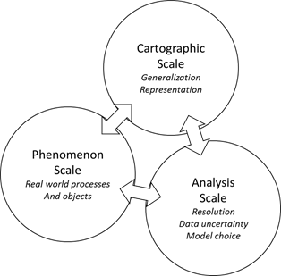
Figure 3.2.1. Three geographic (spatial) scales as defined by Mason (2001).
According to Mason (2001) there are three meanings of "scale" (see figure 3.2.1): i) Cartographic scale refers to the depicted size of a feature on a map relative to its actual size in the world, ii) the Phenomenon scale refers to the size at which human or physical earth structures or processes exist, regardless of how they are studied or represented, and iii) the Analysis scale refers to the size of a unit at which some problem is analyzed (often called resolution).
It is not the intention of this distinction in three scale and their definitions to exclude other concepts, and between the three definitions are also interrelated. The purpose is to highlight what a request of generating a "1:50,000 flood hazard map" actually means. This discussion is focused on spatial scales, while at the end of this section the temporal scale in the context of flood hazard assessment will be briefly discussed.
Cartographic Scale
When determining the cartographic scale at which a flood hazard is represented, a given level of detail is automatically assumed, as we are generally very familiar with the level of detail one expects in a map of a given scale. The expected level of detail comes from the cartographic process of generalization, to create usable maps from ta very complex reality on the earth surface. Generalization can consist of (see e.g. Campbell, 2001):
- selection of certain elements to be shown (e.g. an airport is shown, but a hospital only indicated with a symbol),
- simplification in shape and texture to enhance visibility,
- combination of detailed elements into larger units of information, this often follows a thematic logic, e.g. combine different forest types into one unit "natural vegetation",
- smoothing of boundaries and line elements to enhance readability,
- enhancement of given elements relative to the theme of the map, e.g. enhance touristic sites,
- displacement where two objects are so close together that they overlap at a given scale, and a single object in a location central to the two is shown.
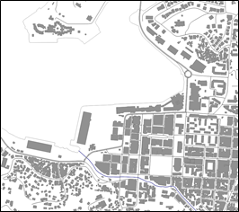
An example of cartographic generalization is given in figure 3.2.2. We are so used to this for topographic information in everyday life that a scale indication has become synonymous for an expected level of generalization.
 |
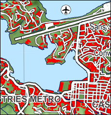 |
Figure 3.2.2. Digitized building footprint in the St Lucia GIS database (left), and generalized topographic map 1:50000 (right).
The 1:50000 topographic map of the islands shows the township boundaries, and road network, but not individual buildings and the roads do not have their true width, but are classified into main roads and secondary roads. Symbols show the presence of specific buildings such as hospitals and schools, with an approximate location. We know this intuitively and the map is conform our expectations, because of the long historical guidelines and developments in cartography that are mainstream. The expectation of the level of information has become inherent to the scale: a 1:100 scale map of a village shows cadaster boundaries if they exist and exact shapes and locations of houses, roads, bridges etc. The cartographic definition of small-scale for few details and strongly generalized information (large scale number, e.g. 1:1000000), and large-scale for abundant detail and little generalization (small scale number, e.g. 1:10000) is often felt to be counter-intuitive. The cartographic scale is directly related to elements and boundaries we can see and measure at the earth surface, without any intervention of a model or method.
When dealing with information that comes from a flood hazard method or model such as listed in section 3.1, this is far less clear. Here we deal with a phenomenon scale and an analysis scale, and the level of detail achieved depends on the method chosen and the quality and level of detail used. The conversion and depiction of the flood hazards results into a Cartographic scale is often an independent step, although it should not be. It is perfectly possible to run a flood model at a low level of detail, using for instance a 90m resolution SRTM DEM, and subsequently depict the results on a high resolution image or air photo, with a scale of for instance 1:500. The level of detail of the image suggests a very precise results where the flood characteristics can be exactly determined at building level, and the model software will calculate a flood depth in for instance mm precision. Any model will give a high calculation precision, but this does not mean the phenomenon can actually be predicted with such precision for a given dataset. This suggests a level of detail to the inexperienced user that is not realistic, leading to false expectations and even wrong decisions. Vice versa, a flood hazard can be determined with a 1m resolution Lidar DEM, using a calibrated model with the best possible dataset, after which the results are generalized to a 1:50000 scale map. This is in principle correct, although maybe useful information is not shown. Furthermore, while a 1m resolution DEM is present, many of the older "upstream catchment" models do not use such data (models in category C1, table 3.1 in section 3.1), but consider 1st order catchments as a unit with average characteristics. These models stem from a time when computers were less powerful and available digital data not common, so they simplify the landscape in a few large elements that are assumed to be homogeneous in characteristics. In other words, the presence of high resolution data does not guarantee a model or method uses it at the level it is available. Thus we have to consider the analysis scale because it has an important effect on the cartographic scale.
Phenomenon scale
Central to geographical sciences is the realization that in order to study a phenomenon most accurately, the scale of analysis must be close to the scale of the phenomenon (Keim et al., 2010). The phenomenon scale refers to the size at which human or physical earth structures or processes exist, regardless of how they are studied or represented. Within an area that is undergoing a flood, there are many detailed hydraulic processes taking place: acceleration of water when it is compressed between houses, flow changing from supercritical to subcritical flow over short distances, water entering a building which affects its dynamics and that of the water surrounding a building, drainage ditches that guide water out of an area, etc. Also upstream there are many detailed hydrological processes that lead a river overflowing: infiltration differences between agricultural fields and natural forests, obstacles that slow down runoff, variations in channel width that change the flow conditions of the discharge. The amount of detail and variation in these processes increases as we "zoom in" and is in principle endless. This has led to studies about the fractal nature of certain processes and phenomena. Within hydrology, there are models that have a resolution smaller than the size of raindrops to study water behavior as particle physics, while others use an entire slopes or catchments as a single homogeneous unit. In other words, conceptually we know a great deal about these processes, but in practice we resort to a specific model to do the calculations for us, because it is essentially impossible to simulate reality on a 1:1 level. Obviously flood hazard modeling on a resolution smaller than a raindrop is completely impractical and likely not at all useful, while flood hazard modeling using catchments as homogeneous units may be useful for large countries or continental scales as flood indicators or early warning but it will be difficult to simulate scenarios that deal with land use changes or conservation methods, and it will be difficult to relate the model results to the built environment.
One of the most important steps related to the analysis scale is therefore the choice of model or method to simulate a flood. From the start of the exercise "create a flood hazard analysis of an area", we swap the reality for a model. This is unavoidable, but it determines all three scales.
The phenomenon scale is mainly a scale on which research is done and within the context of hazard analysis leads to the more practical scale of analysis, which is the translation of the real world into a model analysis context.
Analysis scale
Mason (2001) says about the analysis scale: "[...] the size of the units in which phenomena are measured and the size of the units into which measurements are aggregated for analysis and mapping. It is essentially the scale of understanding of the geographic phenomena. Terms like 'resolution' or 'granularity' are often used as synonyms for the scale of analysis". The underlying idea is that we must study and analyze a phenomenon at a scale in space and time that represents the actual process.
Section 3.1 lists a series of models and organizes them in relation to their function and the processes they are capable of simulating. It should be mentioned that all models mention a preferred scale at which they use and are proven to work in many circumstances is the user community is large. In general a minimum and maximum resolution is indicated. Some are directly related to a GIS system and use raster or vector data as it is available, others require the construction of an input dataset. All models also make sure that they are physically correct, i.e. they adhere to laws of conservation of mass and conservation of momentum. That means that a hydrological balance will be calculated with very little error. However, this is not a guarantee at all for a good prediction.
Uncertainty
A model result is generally discussed in terms of accuracy and precision. Figure 3.2.3 shows the principles of these two terms and how they relate. Be aware that the center of the circles, the 'truth' relates to the exact flood phenomenon in space and time. Changes in accuracy and precision of the model outcome are a result of uncertainty of model input.
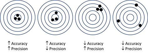
Figure 3.2.3. General diagram to understand the terms precision and accuracy.
Imagine a model calculating the hydrological processes that lead to runoff, the runoff is routed to a riverbed and becomes discharge, which may eventually overflow and cause a flood. All runoff/flood models essentially follow this order of processes. When we keep this in mind we can identify sources of uncertainty (non-exhaustive):
- Choice of input data relative to the location and time of the phenomenon modeled (in this case flash floods): the data itself may be perfectly accurate but measured at a location that is not representative for the area (the 'nearest' rainfall station);
- The rainfall input data may not be actually measured, but a statistical construct representing a rainfall event with a given return period, a so called design event. The design event does generally not resemble a real event in space and time, it only has a statistically correct length, volume and peak intensity;
- Data quality may be an issue. The easiest to understand is the quality of the DEM which can be derived from remote sensing (SRTM, Aster) or from airborne platforms (LiDAR), or from photogrammetry (stereo air photo's) that is later interpolated with a given interpolation method (of which there are many) to obtain a DEM. All of these products have a given vertical accuracy related to their spatial resolution. Since flooding reacts strongly to differences in elevation the DEM quality has a large effect on the result;
- User-data choices: a given model determines a series of input data layers, which are generally derived from basic 'landscape' data, such as soil maps, geomorphological maps and land use/land cover maps. These maps have their own accuracy, they have different cartographic scales, and they are not created for the purpose of flood modeling, but give general information. They have to be translated into hydrological and hydraulic parameters for the model. Sometimes this happens in the model, sometimes this has to be done by the user as preparation. User choices that have to be made in order to run the model could entail: translation of a soil classification map into soil hydrological properties, using average values found in literature; use of a satellite image of a particular moment in time (not corresponding to the moment of flooding) that is converted into land cover classes with an unsupervised classification (which may have between 20 and 30% misclassification), and then translating these classes into their hydrological behavior influencing infiltration and resistance to overland flow; not including effects of tillage and farm operations that influence the hydrology; not knowing if the road is elevated above the landscape which can obstruct water, or the road being deeper that the surrounding terrain so it acts as a temporary channel, making assumptions of the river bed dimensions, etc. In any model there is a long list of assumptions in translating raw data to input data for a model, which affect the uncertainty of the results.
- Model/method generated uncertainty. Uncertainty stemming from the way processes are included: some models generalize a part of the hydrology altogether and simply calculate the fraction of rainfall that turns into runoff (e.g. the CS curve number method). This leads to an uncertainty in runoff percentages: the empirical methods are only tested in certain parts of the world (mostly in the US) and may not be applicable directly to the volcanic soils and tropical environment of the Caribbean islands. Also models are generally highly non-linear and the uncertainty on the end result for a given set of input data differs per model.
Trying to deal with uncertainty and researching its effect on the model result has led to stochastic modeling. Generally we simulate with one set of accepted input data to produce one output (deterministic modeling), but one can also assume a statistical distribution for each input parameter that represents the range of uncertainty of a parameter, and run the model multiple times to generate a large range of possible output (so called realizations). This gives the end-user an idea of the boundaries in which the true outcome exists. While it gives a good idea of the quality of predictions, it is generally not practical in a context of flood mitigation where engineering or planning decisions have to be made.
Calibration, validation
The ultimate goal of modeling flash floods, is to produce a flood hazard assessment, or provide decision support for flood mitigation. Given the sources of uncertainty listed above, tis requires a certain amount of trust in the model or method. This trust can come from using a well proven, worldwide adapted model that has a large user base, and also from calibration and validation when the model is applied to the local circumstances. Calibration of model output against measured values (discharge data, flood levels, community based flood extent maps) is required, and if possible verified against an independent dataset. Because severe floods are also rare, and the circumstances during a flood are such that equipment breaks down, the options are limited. The proper way of modeling follows these steps:
- Choose a model appropriate for the task (see next section) ;
- Collect and create input data;
- Do a sensitivity analysis to understand which parameters for this particular need to be obtained as accurately as possible;
- Calibrate the model for flood circumstances against measured data, if these are not available calibrate against high discharges;
- Validate against independent datasets;
- Translate model results into information useful for stakeholders;
- Present these results on a particular cartographic scale.
The end result is an ensemble of model and data that can be trusted to produce flood hazard analysis and flood mitigation support, for circumstances that are not measured but assumed (e.g. storms with a given return period). This ensemble, model and dataset, needs to be able to give results at a scale useful for the end-user/stakeholder.
Temporal Scale
A flash flood is by nature a fast and abrupt phenomenon, it occurs within hours after a heavy rainfall event, and lasts several hours. It is very dynamic: a map of flood extent, or maximum water levels suggests a still standing pool of water, but the reality is a rapid overflow of the river banks, where people living close to the river are affected immediately, while people living further away perpendicular to the river, or further downstream may have more than an hour to react. A map with a maximum flood level does not mean that that flood level occurs everywhere at the same time, it is a generalization of the process. The same holds for flood recession. On a small scale map such details cannot be shown and the flood dynamics are aggregated to a single flood extent or a combination of flood depth and extent for hazard purposes (see section 3.1).
Agreed Scales for the Caribbean islands
Three scale levels were determined by the World Bank for the analysis of flood hazard on the Caribbean islands. Note that the country of Belize is much larger than the islands, and different scale levels are used (see section 3.4). The (cartographic) scales are defined in table 3.2.1. Furthermore it is possible to distinguish different stakeholder groups and determine what they need and what they can do with the flood hazard information.
Table 3.2.1. Cartographic scales of flood hazard information, the national scale is further elaborated in table 3.2.3.
|
Scale |
Information |
Topography |
Use for: | Do not use for: |
|---|---|---|---|---|
| 1:50000 | National scale flood map, based on flood extent only | Village boundary, generalized roads and rivers | General hazard analysis, focus areas for rapid damage assessment, national planning, prioritizing | Engineering and planning purposes |
| 1:5000 - 1:10000 | Catchment management for flood mitigation, flood characteristics | Building density, road width and type, bridge by location, river channel width and depth | Physical planning and land use planning, early warning, certain forms of conservation and mitigation. | Engineering |
| 1:500-1:1000 | Local scale, section of a catchment, village or part of a community | Individual buildings, walls, roads, bridges, culverts. Exact dimensions hydraulic structures | Engineering of flood limitation structures, bridge and culvert design. Building codes. |
Not useful for hazard zonation analysis. |
This information is generated form a logic of looking at the flood modeling results, bearing in mind the uncertainties discussed above and the model workflow presented in section 3.3. This will give a general results as shown in figure 3.2.4. The resolution of the flood model (the analysis scale) is in the case of the islands done with a 100 m2 resolution (super-use case for catchment management, section XXX) or 400 m2 resolution (national flood hazard analysis). In general building sizes are smaller than 400 m2 and roads and rivers are narrower than 20m. Given the uncertainty in the model results, an area of 10-20 pixels (0.01 km2) is representative for the level of detail of which we can say with certainty it will be flooded. We can determine if groups of houses and stretches of roads are flooded (see fig 3.2.4).
Following this reasoning table 3.2.3 a to c gives advice on how the national flood hazard map can be used, and for which purposes it should not be used.
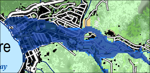
Figure 3.2.4. Detail of the national flood hazard map of St Lucia (Jetten, 2016) as an example of detail. Each pixel of the flooded area is 20x20m. The background is the topographic map 1:50000.
| Stakeholder | Information | Planning | Action |
|---|---|---|---|
| General Public | Flood awareness | General area to avoid - NOT individual property level | What areas require more detailed engineering studies |
| National and local government planning | Preparedness and resilience investment needs. National view of most likely risk | Identify new flood defense and warning schemes. Planning zones definitions | Commission specific detailed studies in high risk areas / catchments |
| National and local government infrastructure | Avoidance areas for new infrastructure. Asset management scenarios | Identify assets at highest risk and mitigation investment required. Investment in assets where damage is greatest | Location and targeting post event repairs. Identify and target maintenance investment |
| National natural resources monitoring agencies | Sensitive regions and locations or river reaches | Identify new information, (data collection) needs e.g. gaging stations | Install new monitoring and flood warning systems. Collect long term flood records |
| National emergency management | Flood hazard communication | Location of evacuation centers and routes. What areas require more detailed engineering studies | Targeting event / incident response |
| Commercial concerns (e.g. agriculture) | Exposure of existing assets | Identify less risky locations for investment | Invest in local protection / preparedness |
| Academia and consultancy | Areas and mechanisms to study further | Targeted research proposals. New data collection | Study, analyze and publish findings relevant to flood risk |
| Insurance | Exposure of portfolio (customers) | New markets or tailored insurance products to risk | Set premiums relative to risk |
| Application scale | Size range (km2) | Application of the NFHM | Suitability | Limitations |
|---|---|---|---|---|
| National | 617 | Yes | National risk assessment | Should represent a good assessment of the hazard at a national scale |
| Catchment | 5 - 100 | Yes | Identifying areas prone to floods, deepest and most frequently | Good assessment of hazard at catchment scale; accuracy will reduce for smaller catchments and sub-catchments. Dynamics of flooding not captured |
| District | 15 - 80 | Yes | Identifying which districts are at risk, or have the most risk | Should represent a good assessment of hazard at district scale |
| Settlements | 0,01 - 10 | Only for the large settlements | Identifying which settlements are at risk, or have the most risk | All cities, some towns, but not villages; see breakdown of settlements in table 3.2.3b |
| Application scale | Size range (km2) | Application of NFHM | Suitability | Limitations |
|---|---|---|---|---|
| City | 1 - 10 | Yes | Identifying which cities are at risk or have the most risk. Can also be used to identify which parts of the city are most at risk | Cities in low lying (flat) areas may not show full risk due to urban artifacts in the topography that are not represented in the DEM |
| Town | 0,1 - 2 | Yes | Identifying which towns are at risk or have the most risk. Can also be used to identify which parts of the towns are most at risk | As above; towns below 1 km2 may not represent full risk |
| Village | 0,01 - 0,1 | Only for the larger villages | Not ideal for this scale and best not used for individual villages (or buildings). |
| Application | Size range (km2) | Application of NFHM | Suitability | Limitations |
|---|---|---|---|---|
| Road | Linear feature (width 10-20m, length range 1 - 10 km) | Limited to planning | Can be used for route planning and avoidance of obvious hazardous areas and to identify the requirement for more detailed flood studies. Also national and district level assessment of road length exposed to flood hazard | Not to be used for road infrastructure design. This requires more detailed hydraulic analysis with more accurate data (DEM) |
| Bridges - Culverts | 10 - 20 m | Limited to planning | Identification of bridges and culverts that might require appraisal for capacity issues and design. | Not to be used for bridge and culvert infrastructure design. This requires more detailed hydraulic analysis. |
| Industrial or housing estate | (1 - 2 km2) | Limited to planning | Identification of estates that may require further detailed assessment or planning zoning control | Only a general assessment of whether a location is exposed to a hazard or not, and the proximity to the hazard is possible at this scale. Quantifying risk may not be possible with any accuracy. |
| Agricultural fields | (0,01 - 0,5 km2) |
|
Identifying fields that may require further detailed assessment | Only a general assessment of whether a location is exposed to a hazard or not, and the proximity to the hazard is possible at this scale. Quantifying risk may not be possible with any accuracy. |
| Buildings | 10 x 10 m | No | Not ideal at this scale and best not used for individual buildings. |
References
Campbell, J. (2001). Map Use and Analysis (4th ed.). New York: McGraw Hill.
Keim, D, Kohlhammer, J. Ellis, G. and Mansmann, F. 2010. Mastering the information age, solving problems with visual analysis. Chapter 5: Space and Time. Printed by Thomas Munzer GMBH, Bad Langensalza. Pp57-86.
Mason, A., 2001. Scales in geography. In International Encyclopedia of the Social & Behavioral Sciences, N.J. Smelser & P.B.Baltes (Eds.).Oxford: Pergamon Press. pp. 13501-13504.