

This use case is part of a series of use cases dealing with the analysis of changing risk.
In the previous use-case you have analyzed the current level of risk, and it was found that in certain parts of the area the risk was too high. This part deals with the formulation of possible risk reduction alternatives, which can be sets of measures that together are aiming to reduce the risk. Three sets are evaluated in this use-case: engineering solutions, ecological solutions and relocation planning. the question is which of these three sets would give us the best risk reduction, and which set would have the best cost-benefit relation. The steps that you need to do for that are explained in this use case.
Keywords:
risk reduction; alternatives; engineering; ecological; relocation; reanalyzing risk; cost estimation; cost-benefit analysis.
| Before you start: | Use case locations: | Uses GIS data: | Authors: |
|---|---|---|---|
| You can first read the procedure on this web-page before downloading the data-set and software and carry out the hands-on training exercise | The use cases in this chapter are related to a hypothetical situation on one of the small Caribbean islands |
Yes, the uses cases are accompanied by GIS exercises that utlize the ILWIS GIS software Download the data (save iink as) Download the software as a Zip file (use save link as) |
Cees van Westen |
Introduction:
After knowing how you calculate the loss using the script Loss_calculation and how to generate the risk curve using the script Risk_calculation, as was explained in the previous use case (4.2), we will now evaluate the possibilities for risk reduction. The results of the previous use-case (4.2) show the resulting loss values for the three hazard types (flooding, debrisflows and landslides) for different return periods (1 in 20 years, 1 in 50 years and 1 in 100 years). The results show the losses for the 19 administrative units in the study area. As you can see (see resulting table from the previous exercise) the results show that in some of the administrative units the risk is higher than in others. For instance administrative units 4,5 and 6 have high potential losses for all three hazards. Unit 8 has only flood losses. Unit 13 has predominantly landslide losses. You can also see that the average annual losses for the entire area, based on the three hazards are high: 173 thousand Dollars per year. Therefore it is important to take action and plan for risk reduction measures to reduce the risk
A similar calculation can be done for population losses. The results for that also show that in some of the administrative units the population losses are high. This is the basis for evaluating which risk reduction alternatives would be the best to implement.
Objectives:
In this exercise we will identify three risk reduction alternatives and reanalyse the risk, the calculate the risk reduction (which is the average annual risk after the implementation minus the current average annual risk). We will later also make an estimation of the costs for the alternatives and carry out a cost-benefit analysis.
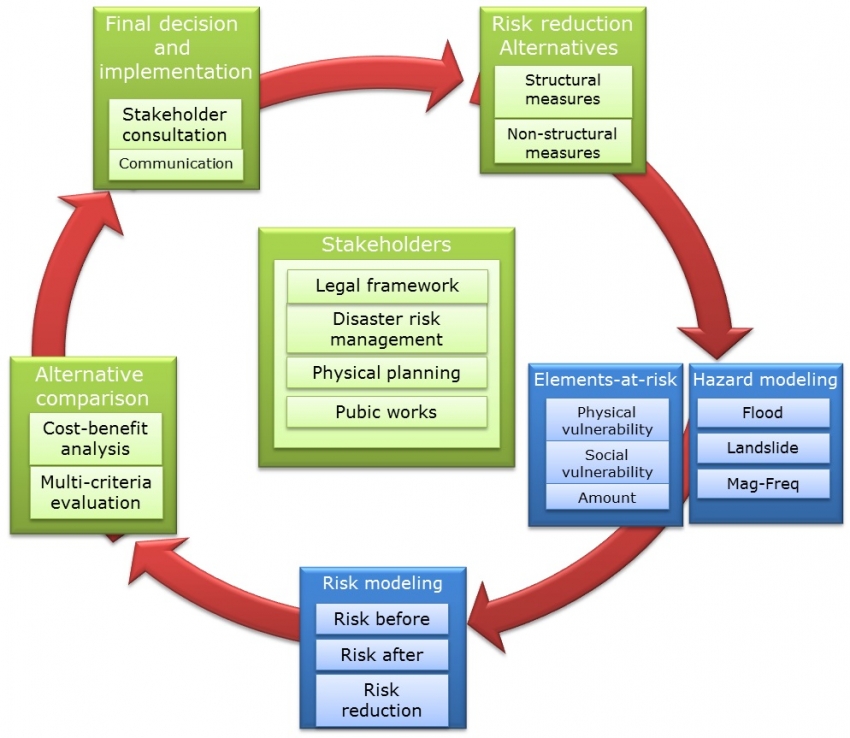
Flowchart:
Use case study area description:
The use-case deal with the same mountainous area along a coast in a Caribbean setting as was explained in use-case 4.1.
Problems definition and specifications:
After consultation meetings with the stakeholders the following three risk reduction alternatives have been defined:
Alternative 1: Engineering measures
This alternative aims at constructing active and passive control works using engineering measures:
- Take out the soil in the landslide prone areas
- Create storage basins that will retain the floods and debrisflows
- Create water channels to guide the water
- Create a monitoring and early warning system
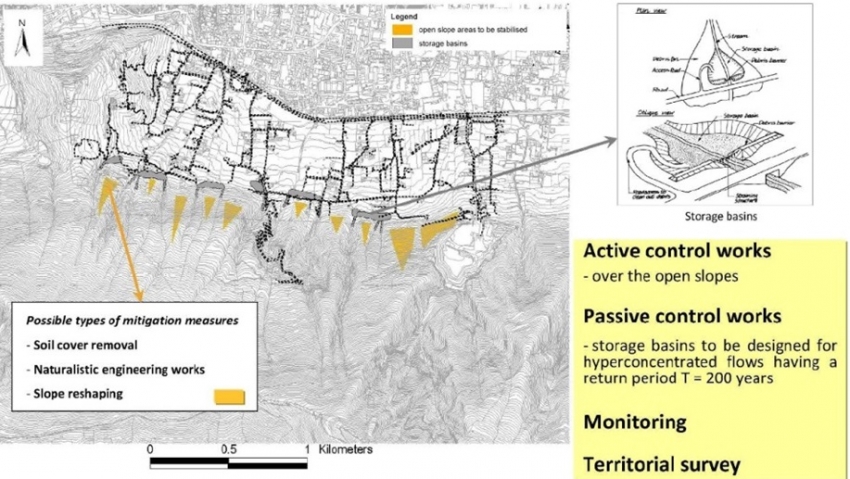
We have made new land parcel maps for the alternative, and new hazard intensity maps. For the alternative 1 we assume that the engineering works will block all debris flows and floods for return periods up to 100 year. For return period of 200 years the engineering solutions might not be sufficient, and the storage basins will overflow.
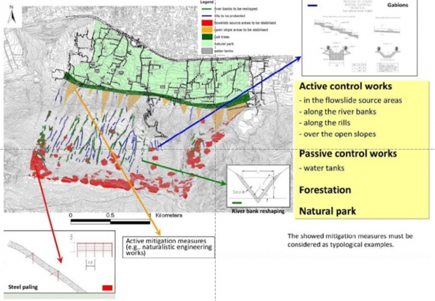
Alternative 2: Ecological solutions
This alternative aims at constructing active and passive control works using ecological solutions:
- Take out the soil in the landslide prone areas
- Use soil nailing in the upper slope to reduce the landslide susceptibility
- Create water tanks that will retain some of the the floods
- Create water channels to guide the water
- A barrier of oak trees that will retain some of the debrisflows and mudflows
- Create a natural park which will stop further development
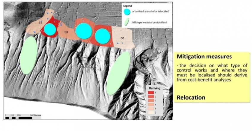
Alternative 3: Relocation of the most endangered buildings
This alternative aims at relocation the residential population from the most endangered administrative units indicated as blue spots in the figure :
- Evacuation of the people requires that they have to be financially compensated, and that they are willing to collaborate, otherwise lengthy procedures and lawsuits are required which may take a lot of time.
Data requirements:
The data requirement for the use case are illustrated in the animated presentation (click the image to start this in a new window. There you can click on any of the hyperlinks and navigate through the different risk reduction alternatives, and the hazard and elements-at-risk maps used for them) .

Analysis steps:
Step 1: Loss analysis of the new situation after implementing the risk reduction alternatives
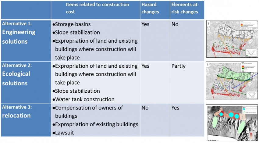
The first step to do is to reanalyze the losses , but now for the new situations that would exist if the risk reduction alternatives would be implemented. In the animation above you have seen the various input maps that are required for each of the three alternatives. They are also summarized in the three table below, whihc gives the example for alternative 1. As you can see from the animation, depending on the proposed risk reduction alternative, both hazard maps and elements-and-risk maps should be updated.
For alternative 1: both hazard maps and elements-at-risk maps should be updated. Constructing the engineering measures will greatly reduce the flood, debrisflow and landslide hazards. However, as the most eastern watershed is not considered in the plans, there the flood and debris flow hazard will remain the same. The engineering works have been designed for a return period of 100 years. Therefore we have also modelled the 1 in 200 year event, and for this situation the engineering works will be partly overtopped. The construction of the storage basins requires to change the land use and relocate some of the houses which are in the location of the storage basins. Therefore also a new elements-at-risk map is needed.
For alternative 2: also both hazard maps and elements-at-risk maps should be remade, as they both will change as a consequence of the risk reduction alternative. The plantation of the protective forest will greatly reduce the hazards, however, not as much as the construction of the engineering works. It will also take a number of years before the trees in the protective forest are tall enough to have their full protection function. Also for the plantation of the protective forest some land parcels will have to cgange their land use and some buildings have to be relocated.
For alternative 3 (relocation) only the elements will change. This alternative doesn't involve the reduction of hazards, but only the reduction of the exposed elements-at-risk (buildings). therefore the same hazard maps can be used as for the current situation.
|
Hazard type |
Return period |
Intensity measure or spatial probability |
Present situation: |
Alternative 1: Engineering measures |
Alternative 2: Ecological solutions |
Alternative 3: Relocation |
|---|---|---|---|---|---|---|
|
Landslide |
20 |
Spatial Probability |
LS_SP_20_A0 |
LS_SP_20_A1 |
LS_SP_20_A2 |
LS_SP_20_A3 |
|
Landslide |
50 |
Spatial Probability |
LS_SP_50_A0 |
LS_SP_50_A1 |
LS_SP_50_A2 |
LS_SP_50_A3 |
|
Landslide |
100 |
Spatial Probability |
LS_SP_100_A0 |
LS_SP_100_A1 |
LS_SP_100_A2 |
LS_SP_100_A3 |
|
Landslide |
200 |
Spatial Probability |
LS_SP_200_A0 |
LS_SP_200_A1 |
LS_SP_200_A2 |
LS_SP_200_A3 |
|
Debrisflow |
20 |
Impact pressure |
DF_IP_020_A0 |
DF_IP_20_A1 |
DF_IP_20_A2 |
DF_IP_20_A3 |
|
Debrisflow |
50 |
Impact pressure |
DF_IP_050_A0 |
DF_IP_50_A1 |
DF_IP_50_A2 |
DF_IP_50_A3 |
|
Debrisflow |
100 |
Impact pressure |
DF_IP_100_A0 |
DF_IP_100_A1 |
DF_IP_100_A2 |
DF_IP_100_A3 |
|
Debrisflow |
200 |
Impact pressure |
|
DF_IP_200_A1 |
DF_IP_200_A2 |
|
|
Flood |
20 |
Water depth |
FL_DE_020_A0 |
FL_DE_20_A1 |
FL_DE_20_A2 |
FL_DE_20_A3 |
|
Flood |
50 |
Water depth |
FL_DE_050_A0 |
FL_DE_50_A1 |
FL_DE_50_A2 |
FL_DE_50_A3 |
|
Flood |
100 |
Water depth |
FL_DE_100_A0 |
FL_DE_100_A1 |
FL_DE_100_A2 |
FL_DE_100_A3 |
|
Flood |
200 |
Water depth |
|
FL_DE_200_A1 |
FL_DE_200_A2 |
|
|
Land Parcel maps |
|
LP_2014_A0_S0 |
LP_2014_A1_S0 |
LP_2014_A2_S0 |
LP_2014_A3_S0 |
|
Similarly as the analysis which was done for the current risk we are doing this analysis in two steps:
- Loss analysis for each individual combination of hazard set (for a given date, hazard type and return period) and elements-at-risk (the land parcel map for the given risk reduction alternative).
- Risk analysis by combining the loss results for different hazards and return periods.
Loss analysis can be automated with a script Loss_calculation for that.
Step 2: Risk analysis of the new situation after implementing the risk reduction alternatives
The risk analysis which was done using a scrip Risk_calculation (see previous use cases) can now also be done for the different scenarios. We assume that flooding, landslides and debrisflows are depending on the same trigger, so we take the maximum losses for a given area from one of the three hazards. We assume that if a triggering events occurs it may trigger either landslides, flashfloods or debrisflows, and the area affected by one would lead to a certain amount of losses. If another event also happens it will not cause twice the same damage.
The input data for the risk analysis is handled through the scrip Risk_calculation_input. For running the alternatives 1 to 3 the following information should be available:
Note that we first calculate the current risk, and then calculate the risk for the three alternatives. The results show the average annual risk before and after the implementation of the alternative, and the difference, which is the annual risk reduction. This will be used in the cost-benefit analysis and is called the Benefit for each alternative.
Step 3: Cost estimation of the alternatives.
After calculating the risk curves and annual risk for the current situation and for one or more of the three alternatives, you can analyze which of the alternatives leads to the highest risk reduction (the largest benefit). However, the costs for the alternative might be much higher. Therefore it is important to also analyse the cost-benefit relation.
In order to do that you need to estimate the costs for each of the alternatives. For that you need to analyse:
- The initial investment costs
- The period over which these investment costs are made
- In which year after the start of the construction are the benefits achieved.
- The annual maintenance costs
- The total duration of the project. In our case we will use a project lifetime of 50 years.
The initial investment costs are composed of all the costs needed to carry out the alternative. The implementation of each alternative will have a number of components that each costs money. The first part of the analysis is to identify all the individual cost options. The table below shows which aspects are considered for estimating the costs:
|
Items related to construction cost |
Time of construction |
Benefit starts |
Annual Maintenance |
|
|---|---|---|---|---|
|
Alternative 1: engineering solutions |
|
3 years |
4th year |
From year 4 |
|
Alternative 2: Ecological solutions |
|
3 years |
From 4th year with 100% benefit in 10th year |
From year 2 |
|
Alternative 3: Relocation |
|
10 years |
100% benefit starts from 11th year |
From year 11 |
For each of these items you need to make an estimation. The costs estimation can be done in the following ways:
- Calculating the area of land that will change. You can do that using the building maps or the land parcel maps of the present situation and of the alternatives (e.g. LP_2014_A0 as land parcel map of the current situation). This map also has value information and information on the number of people. When you overlay these with the land parcel map for the alternative (e.g. LP_2014_A1 for the parcel map of the first alternative) you can calculate how much area of land will change and their values.
- You can also calculate the area of the land that is converted from the current situation to for example the tree belt under Alternative 2, or the number of retention basin under Alternative 1. You can then use values per m2 in the calculation.
- Make an estimation of the unit costs per m2 that you are using in the analysis, or ask the staff for these values. See also the suggested values on the right side
- Prepare an Excel sheet in which you make a line for each year, and a column for each of the components of the cost analysis. See the example below in the animation.
Step 4: Cost-Benefit analysis
 The following animation shows the steps required for the Cost-Benefit analysis. Follow the individual steps using an Excel sheet in which you do the actual calculations.
- Prepare an Excel sheet in which you make a line for each year, and a column for each of the components of the cost analysis
- After filling in the values in the Excel sheet you can also calculate the overall costs per year for each of the alternatives (the columns: Total)
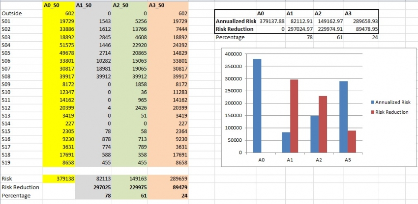
- Calculate the Risk Reduction (as the annualized risk for the current situation minus the annualized risk for the alternative) for the 3 alternatives.
- Decide in which year the Risk Reduction will actually start. It may be possible that in the first years you have investments, but no risk reduction yet, as the alternative to reduce the risk is not finished.
- Think about this for the 3 alternatives and decide in which year we will actually reach the risk reduction.
- In the Excel sheet add for each of the alternatives a column, called Risk Reduction for each of the scenarios.
- In the Excel sheet calculate the Incremental Benefits, by Calculating the difference between the Risk Reduction and the total of the costs per year. For the first years these values might be negative
- In the Excel worksheet to the right of the table make a cell NPV ( Net Present Value) ;
- In the cell next to it insert the name Interest rate (which is the same as discount rate) and enter the value of : 10 %.
- In Excel: Click in your “NPV†cell and Insert Function; select Financial Functions.
- Select: NPV
- The Function Arguments Box opens ( see figure below);
- Select for Interest Rate 6%
- For value 1: select the whole column down all the incremental benefits; starting at year 1 up to year 40.
- Click OK
The Excel sheet looks like this:
- Repeat the NPV calculation, but now with different discount rates
Now we are going to calculate the Internal rate of return. The Internal Rate of Return is the discount rate/interest rate at which the NPV=0
- In Excel: Click Insert Function and select Financial Functions.
- Select: IRR
- The Function Arguments Box opens;
- Read the HELP file
- For values: select the whole column down all the incremental benefits; starting at year 1 up to year 40.
- Click OK.
Now we will compare the NPV and IRR values for the various risk reduction alternatives.
- Calculate the NPV and IRR for the three alternatives. Calculate the NPV for 3 interest rates
- Compare the results.
- Decide which of the three alternatives is the best based on the cost-benefit evaluation.
|
|
NPV at 5 % interest rate |
NPV at 10 % interest rate |
NPV at 20 % interest rate |
IRR |
|---|---|---|---|---|
|
Alternative 1 |
|
|
|
|
|
Alternative 2 |
|
|
|
|
|
Alternative 3 |
|
|
|
|
Results:
The results of the average annual risk calculation for the three alternatives is presented below:
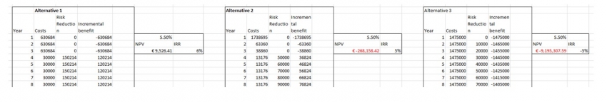
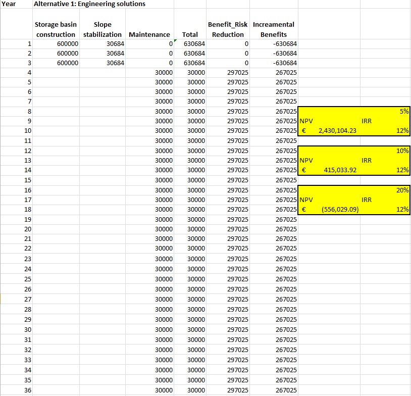
The results of the Cost-Benefit Analysis for Alternative 1 is:
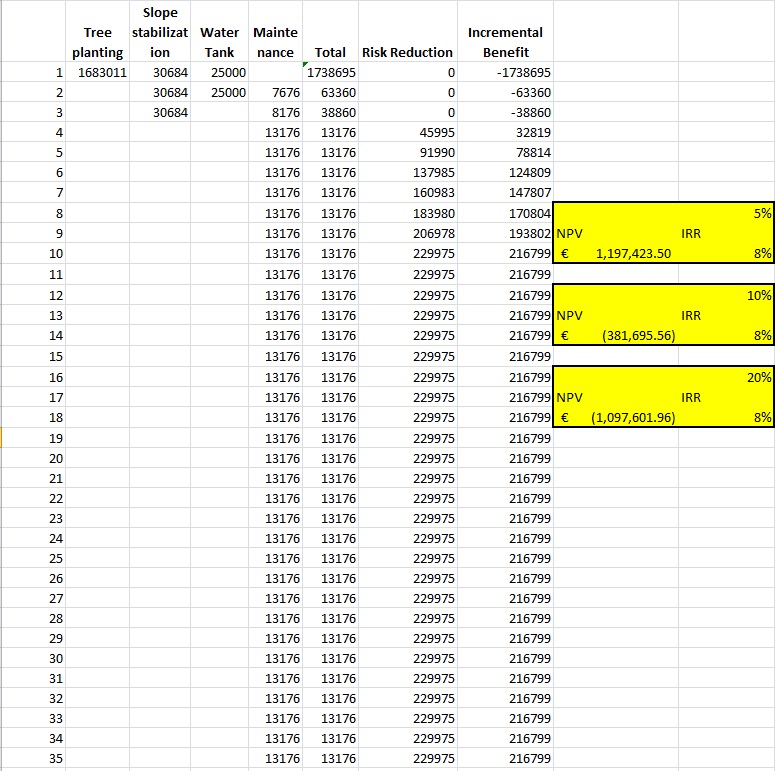
The results of the Cost-Benefit Analysis for Alternative 2 is:
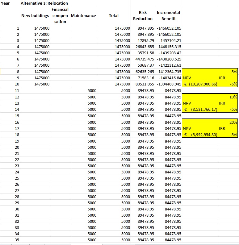
The results of the Cost-Benefit Analysis for Alternative 3 is:
The final results are shown in the table below:
|
|
NPV at 5% Interest Rate |
NPV at 10% Interest Rate |
NPV at 20% Interest Rate |
IRR |
|---|---|---|---|---|
|
Alternative 1: Engineering solutions |
€ 2,430,104.23 |
€ 415,033.92 |
- € 556,029.09 |
12% |
|
Alternative 2: Ecological solutions |
€ 1,197,423.50 |
- € 381,695.56 |
- € 1,097,601.96 |
8% |
|
Alternative 3: Relocation |
- € 10,207,900.66 |
- € 8,531,766.17 |
- € 5,992,954.80 |
-5% |
This means that alternative 3 is always the worst one": the NPV values are always negative. Alternative 1 (Engineering solutions) is the best one, although the differences with alternative 2 (Ecological solutions) are not so very high.
Which alternative would be selected is not only depending on the Cost-Benefit analysis . Also many other factors might play a role, and the stakeholders might have other reasons why they would prefer one particular alternative. Therefore a Multi-Criteria evaluation would be the best next step, in which stakeholders can bring in other indicators (social, environmental, legislation, support by population etc.) and wight them against the risk related indicators and cost-benefit related indicators.
Conclusions:
Which alternative would be selected is not only depending on the Cost-Benefit analysis . Also many other factors might play a role, and the stakeholders might have other reasons why they would prefer one particular alternative. Therefore a Multi-Criteria evaluation would be the best next step, in which stakeholders can bring in other indicators (social, environmental, legislation, support by population etc.) and wight them against the risk related indicators and cost-benefit related indicators.