

By:
Introduction
Risk is defined as the probability of harmful consequences, or expected losses (deaths, injuries, property, livelihoods, economic activity disrupted or environment damaged) resulting from interactions between natural or human-induced hazards and vulnerable conditions (UN-ISDR, 2009, EC, 2011). Risk can presented conceptually with the following basic equation indicated in Figure 1
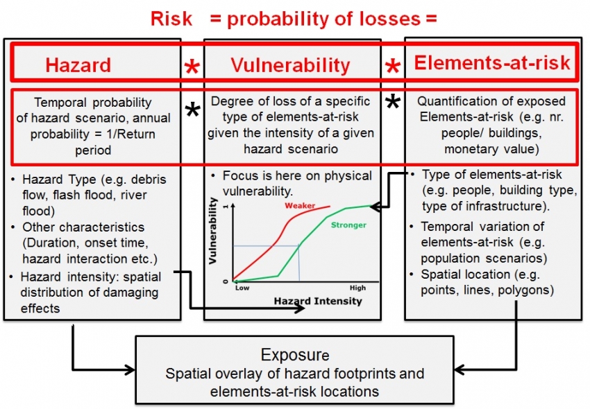
Figure 1: Schematic representation of risk as the multiplication of hazard, vulnerability and quantification of the exposed elements-at-risk. The various aspects of hazards, vulnerability and elements-at-risk and their interactions are also indicated. This framework focuses on the analysis of physical losses, using physical vulnerability data.
Risk assessment is a process to determine the probability of losses by analyzing potential hazards and evaluating existing conditions of vulnerability that could pose a threat or harm to property, people, livelihoods and the environment on which they depend (UN-ISDR, 2009). ISO 31000 (2009) defines risk assessment as a process made up of three processes: risk identification, risk analysis, and risk evaluation. Risk identification is the process that is used to find, recognize, and describe the risks that could affect the achievement of objectives. Risk analysis is the process that is used to understand the nature, sources, and causes of the risks that have been identified and to estimate the level of risk. It is also used to study impacts and consequences and to examine the controls that currently exist. Risk evaluation is the process that is used to compare risk analysis results with risk criteria in order to determine whether or not a specified level of risk is acceptable or tolerable.
Risk mapping for natural hazard risk can be carried out at a number of scales and for different purposes. Table 1 gives a summary. In the following sections four methods of risk mapping will be discussed: Quantitative risk assessment (QRA), Event-Tree Analysis (ETA), Risk matrix approach (RMA) and Indicator-based approach (IBA).
Table 1: Indication of scales of analysis with associated objectives and data characteristics (approaches: QRA = Quantitative risk assessment, EVA = Event-Tree Analysis, RMA = Risk matrix approach, IBA = Indicator-based approach)
|
Scale of analysis |
Scale |
Possible objectives |
Possible approaches |
|---|---|---|---|
|
International, Global |
< 1 : 1 million |
Prioritization of countries/regions; Early warning |
Simplified RMA & IBA |
|
Small: provincial to national scale |
< 1:100,000 |
Prioritization of regions; Analysis of triggering events; Implementation of national programs; Strategic environmental assessment; Insurance |
Simplified EVA, RMA & IBA |
|
Medium: municipality to provincial level |
1:100000 to 1:25000 |
Analyzing the effect of changes; Analysis of triggering events; Regional development plans |
RMA / IBA |
|
Local: community to municipality |
1:25000 to 1:5000 |
Land use zoning; Analyzing the effect of changes; Environmental Impact Assessments; Design of risk reduction measures |
QRA / EVA / RMA IBA |
|
Site-specific |
1:5000 or larger |
Design of risk reduction measures; Early warning systems; detailed land use zoning |
QRA / EVA / RMA |
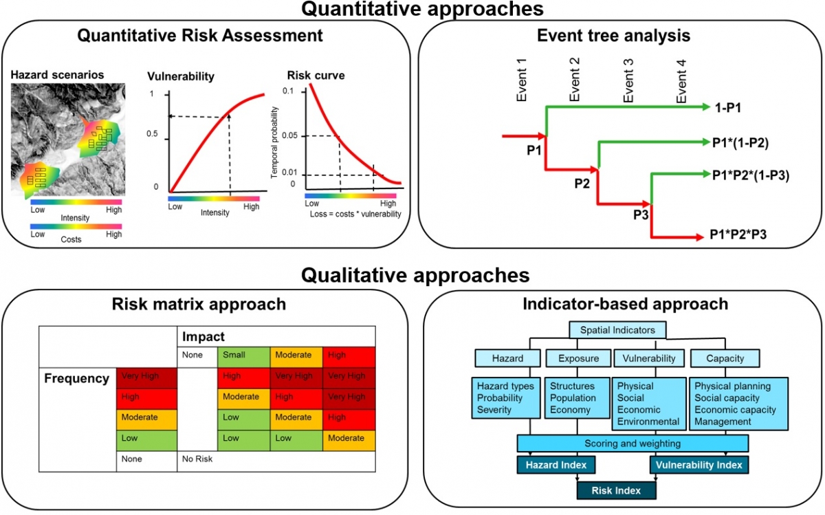
Figure 2: Components relevant for risk assessment, and the four major types of risk mapping that are presented in this section.
Quantitative Risk Assessment
If the various components of the risk equation can be spatially quantified for a given set of hazard scenarios and elements-at-risk, the risk can be analyzed using the following equation:
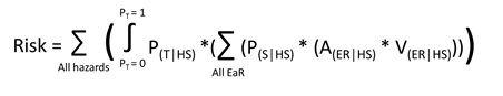
In which:
P(T│HS) = the temporal probability of a certain hazard scenario (HS). A hazard scenario is a hazard event of a certain type (e.g. flooding) with a certain magnitude and frequency;
P(S│HS) = the spatial probability that a particular location is affected given a certain hazard scenario;
A(ER│HS) = the quantification of the amount of exposed elements-at-risk, given a certain hazard scenario (e.g. number of people, number of buildings, monetary values, hectares of land) and
V(ER│HS) = the vulnerability of elements at risk given the hazard intensity under the specific hazard scenario (as a value between 0 and 1).
The method is schematically indicated in Figure 3. GIS operations are used to analyze the exposure as the intersection between the elements-at-risk and the hazard footprint area for each hazard scenario. For each element-at-risk also the level of intensity is recorded through a GIS-overlay operation. These intensity values are used in combination with the element-at-risk type to find the corresponding vulnerability curve, which is then used as a lookup table to find the vulnerability value. The way in which the amount of elements-at-risk are characterized (e.g. as number of buildings, number of people, economic value) also defines the way in which the risk is calculated. The multiplication of exposed amounts and vulnerability should be done for all elements-at-risk for the same hazard scenario. The results are multiplied with the spatial probability that the hazard footprint actually intersects with the element-at-risk for the given hazard scenario P(S│HS) to account for uncertainties in the hazard modelling. The resulting value represents the losses, which are plotted against the temporal probability of occurrence for the same hazard scenario in a so-called risk curve. This is repeated for all available hazard scenarios. At least three individual scenarios should be used, although it is preferred to use at least 6 events with different return periods (FEMA, 2004) to better represent the risk curve. The area under the curve is then calculated by integrating all losses with their respective annual probabilities. It is possible to create risk curves for the entire study area, or for different spatial units, such as administrative units, census tracks, road or railway sections etc. Risk can be presented in a number of different ways, depending on the objectives of the risk assessment (Birkmann, 2007). Risk can expressed in absolute or relative terms. Absolute population risk can be expressed as individual risk (the annual probability of a single exposed person to be killed) or as societal risk (the relation between the annual probability and the number of people that could be killed). Absolute economic risk can be expressed in terms of Average Annual Loss, Maximum Probable Loss, or other indices that are calculated from a series of loss scenarios, each with a relation between frequency and expected monetary losses (Jonkman, van Gelder and Vrijling, 2002)
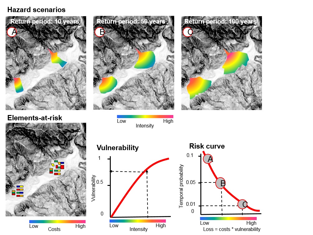
Figure 3: Schematic representation of Quantitative Risk Assessment. Click to enlarge.
The components that are involved in risk assessment have a high degree of uncertainty. Aleatory uncertainty is associated with the variation of the input data used in the risk assessment. For example the variations in soil characteristics used to model landslide probability, surface characteristics, building characteristics etc. These are normally incorporated in probabilistic risk analysis (Bedford and Cook, 2001) which calculates thousands of hazard and risk scenarios taking the variations of the input factors and calculating exceedance probabilities using techniques such as Monte Carlo simulation. Epistemic uncertainty refers to uncertainty associated with incomplete or imperfect knowledge about the processes involved, and lack of sufficient data. This is often a serious problem as there may not be enough data available to determine individual hazard scenarios, or there are no vulnerability curves for the types of elements-at-risk within the study area. Probabilistic risk assessment takes into account all possible hazard scenarios and the uncertainty of the input factors, by running thousands of loss scenarios, and calculate eventually the loss exceedance curve. For a number of hazards, such as landslides or flooding, it is very complicated to develop a large number of hazard scenarios due to the large epistemic uncertainty caused by lack of data. In such cases uncertainty can be taken into account using the method illustrated in Figure 4. In this method data are used showing the range of possible values for the temporal probability, spatial probability, intensity of the hazard, value of the elements-at-risk and vulnerability. The uncertainty range in the temporal probability of the hazard scenario is reflected by a range of possible values on the Y-axis of the risk curve. The uncertainty in the hazard intensity (e.g. water height for flooding, impact pressure for landslides) combined with the uncertainty in the vulnerability curve will results in larger uncertainty ranges in vulnerability, which are then multiplied with the uncertainty range of the quantification of elements-at-risk (e.g. building costs). This then gives a range of values for the expected losses. So instead of a single point in the risk curve, each hazard scenario will result in a rectangle, defined by the variation in probability and losses. The upper right corners of the rectangle are connected to provide the most pessimistic risk curve, and the lower right corners are connected to provide the most optimistic risk curve. When calculating the area under the curves it is then possible to show the range in annual expected losses.
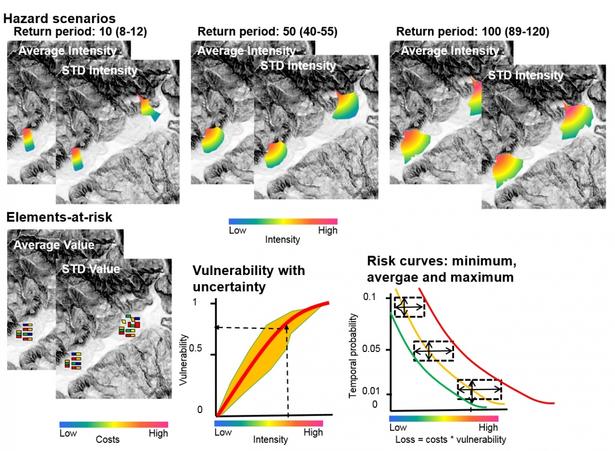
Figure 4: Method for including uncertainty in Quantitative Risk Analysis in cases where it is not possible to define many hazard scenarios. Click to enlarge.
The animation below gives an example of a quantitative risk assessment for buildings that are threatened to flooding with three different scenarios, each with a different probability of occurrence (2 years, 10 years and 50 years). In this simple example there are 3 elements at risk only (buildings) that are of two types. Type-1 buildings are weaker in construction than type-2 buildings. Based on past occurrences of flooding a relation has been made between the water depth and the degree of damage using vulnerability curves (explained in chapter 5, Section 5.3). This means that with the same water depth type-1 buildings will suffer more damage than type-2 buildings. The vulnerability curves presented in animation are hypothetical ones, but are the crucial component in the risk assessment. The three hazard scenarios will affect the three buildings in a different way. The small table in the animation indicates the water depth that can be expected for the three houses related to the three scenarios
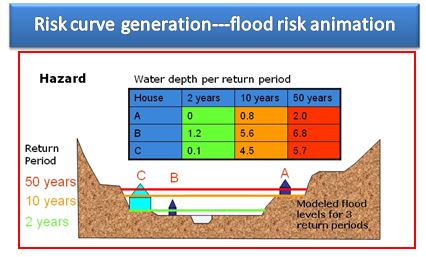
Figure 5: Step-by-step animation of risk assessment illustrated for flooding. Click to start the animation in a new window
Event-tree approaches
A number of hazard may occur in chains: one hazard causes the next. These are also called domino effects, or concatenated hazards. These are the most problematic types to analyze in a multi-hazard risk assessment. The best approach for analyzing such hazard chains is to use so-called event-trees. An event tree is a system which is applied to analyze all the combinations (and the associated probability of occurrence) of the parameters that affect the system under analysis. All the analyzed events are linked to each other by means of nodes (See Figure 6) all possible states of the system are considered at each node and each state (branch of the event tree) is characterized by a defined value of probability of occurrence.
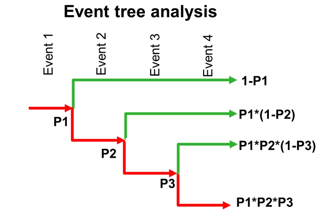
Figure 6: Schematic representation of an event-tree analysis.
The figure below gives an examples of an event tree for a situation where a rockfall in a lake may trigger a flood wave that would impact a village (from Lacasse et al., 2008)

Figure 7: Bayesian Event tree for tsunami propagation, given that rock slide in Aknes has occurred (V= rockslide volume, R=run-up height). From Lacasse et al., 2008) Click to enlarge.
Risk matrix approach
Risk assessments are often complex and do not allow to develop a full numerical approach, since many aspects are not fully quantifiable or have a very large degree of uncertainty. This may be related to the difficulty to define hazard scenarios, map and characterize the elements-at-risk, or define the vulnerability using vulnerability curves. In order to overcome these problems the risk is often assessed using so-called risk matrices or consequences-frequency matrices (CFM), which are diagrams with consequence and frequency classes on the axes (See Figure 8). They permit to classify risks based on expert knowledge with limited quantitative data (Haimes, 2008; Jaboyedoff et al., 2014). The risk matrix is made of classes of frequency of the hazardous events on one axis, and the consequences (or expected losses) on the other axis. Instead of using fixed values, the use of classes allows for more flexibility and incorporation of expert opinion. Such methods have been applied extensively in natural hazard risk assessment, e.g. in Switzerland (Jaboyedoff et al., 2014). This approach also permits to visualize the effects and consequences of risk reduction measures and to give a framework to understand risk assessment. The system depends on the quality of the group of experts that are formed to identify the hazard scenarios, and that carry out the hazard filtering and ranking in several sub-stages characterized by frequency (probability) and impact classes and their corresponding limits (Haimes, 2008).
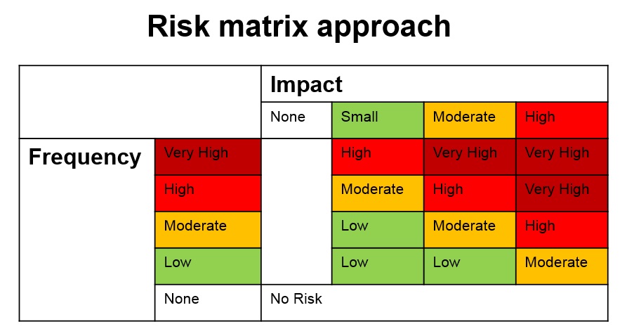
Figure 8: Example of the risk matric approach, which consists of a matrix with classes of frequency (of the hazardous event) and the consequences.
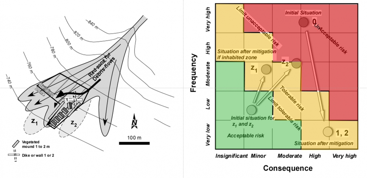
Figure 9: Example of potential building area in a high hazard area and illustration of the proposed solutions. The risk matrix is used to represent the degree of risk. The scope of tolerable risk (yellow) is between the limits of tolerance and of acceptability. The initial situation 0 is a combination of very high frequency of debris flows with a high impact. After construction of a deflection dike or wall the frequency doesn't change but the impact decreases considerably. The areas Z1 and Z2 on the other hand will get a higher frequency of occurrence and higher consequence as a result of the mitigation works (Jaboyedoff et al., 2014). Click to enlarge.
Indicator-based Approach
There are many situations where the (semi)-quantitative methods for risk mapping are not appropriate. This could be because the data are lacking to be able to quantify the components, such as hazard frequency, intensity, and physical vulnerability. For instance when the risk assessment is carried out over large areas, or in areas with limited data. Another reason is that one would like to take into account a number of different components of vulnerability that are not incorporated in (semi-) quantitative methods, such as social vulnerability, environmental vulnerability and capacity. In those cases it is common to follow an indicator-based approach to measure risk and vulnerability through selected comparative indicators in a quantitative way in order to be able to compare different areas or communities. The process of disaster risk assessment is divided into a number of components, such as hazard, exposure, vulnerability and capacity (See Figure 10), through a so-called criteria tree, which list the subdivision into objectives, sub-objectives and indicators. Data for each of these indicators are collected at a particular spatial level, for instance by administrative units. These indicators are then standardized (e.g. by reclassifying them between 0 and 1), weighted internally within a sub-objective and then the various sub-objectives are also weighted amongst themselves. Although the individual indicators normally consist of quantitative data (e.g. population statistics), the resulting vulnerability, hazard and risk results are scaled between 0 and 1. These relative data allows to compare the indicators for the various administrative units. These methods can be carried out at different levels, ranging from local communities (e.g. Bollin and Hidajat, 2006) cities (Greiving et al, 2006) to countries (Van Westen et al., 2012).

Figure 10: Risk Indicator based approach.
The approaches are mostly based on the development of so-called risk indices, and on the use of spatial multi criteria evaluation. One of the first attempts to develop global risk indicators was done through the Hotspots project (Dilley et al. 2005). In a report for the Inter-American Development Bank, Cardona (2005) proposed different sets of complex indicators for benchmarking countries in different periods and to make cross-national comparisons. Four components or composite indicators reflect the principal elements that represent vulnerability and show the advances of different countries in risk management: Disaster Deficit Index, Local Disaster Index, Prevalent Vulnerability Index and Risk Management Index. Each index has a number of variables that are associated with it and empirically measured. The DDI can be considered as an indicator of a country's economic vulnerability to disaster. Information on using the Disaster Risk Index for Belize can found here: https://www.imf.org/external/np/seminars/eng/2013/caribbean/pdf/be .Peduzzi et al. (2005; 2009) have developed global indicators, not on the basis of administrative units, but based on gridded maps. The Disaster Risk Index (UN-ISDR, 2005b) combines both the total number and the percentage of killed people per country in large- and medium-scale disasters associated with droughts, floods, cyclones and earthquakes. In the DRI, countries are indexed for each hazard type according to their degree of physical exposure, their degree of relative vulnerability, and their degree of risk. Also at local scale risk indices are used, often in combination with spatial multi criteria evaluation (SMCE). Castellanos and Van Westen (2007) present an example of the use of SMCE for the generation of a landslide risk index for the country of Cuba, generated by combining a hazard index and a vulnerability index. The hazard index is made using indicator maps related to triggering factors (earthquakes and rainfall) and environmental factors. The vulnerability index was made using five key indicators: housing condition and transportation (physical vulnerability indicators), population (social vulnerability indicator), production (economic vulnerability indicator) and protected areas (environmental vulnerability indicator). The indicators were based on polygons related to political-administrative areas, which are mostly at municipal level. Each indicator was processed, analysed and standardized according to its contribution to hazard and vulnerability. The indicators were weighted using direct, pair wise comparison and rank ordering weighting methods and weights were combined to obtain the final landslide risk index map. The results were analysed per physiographic region and administrative units at provincial and municipal levels. Another example at the local level is presented by Villagrán de Leon (2006) which incorporates 3 dimensions of vulnerability, the scale or geographical level (from human being to national level), the various sectors of society, and 6 components of vulnerability. The method uses matrices to calculate a vulnerability index, which was grouped in qualitative classes (high, medium and low).
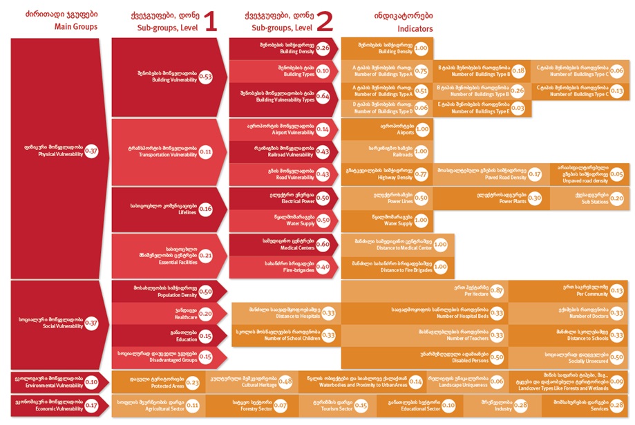
Figure 11: Example of the use of indicators in a Spatial Multicriteria Evaluation for the country of Georgia (Van Westen et al., 2012) Click to enlarge.
Conclusions
The four methods for risk assessment that were treated in this chapter all have certain advantages and disadvantages, which are summarized in Table 3. The Quantitative Risk Assessment method is the best for evaluating several alternatives for risk reduction, through a comparative analysis of the risk before and after the implementation followed by a cost-benefit analysis. The event-tree analysis is the best approach for analyzing complex chains of events and the associated probabilities. Qualitative methods for risk assessment are useful as an initial screening process to identify hazards and risks. They are also used when the assumed level of risk does not justify the time and effort of collecting the vast amount of data needed for a quantitative risk assessment, and where the possibility of obtaining numerical data is limited.The risk matrix approach is often the most practical approach as basis for spatial planning, where the effect of risk reduction methods can be seen as changes in the classes within the risk matrix. The indicator-based approach, finally, is the best when there is not enough data to carry out a quantitative analysis, but also as a follow-up of a quantitative analysis as it allows to take into account other aspects than just physical damage.
Table 2: Advantages and disadvantages of the four risk assessment methods discussed.
|
Method |
Advantages |
Disadvantages |
|---|---|---|
|
Quantitative risk assessment (QRA) |
Provides quantitative risk information that can be used in Cost-benefit analysis of risk reduction measures. |
Very data demanding. Difficult to quantify temporal probability, hazard intensity and vulnerability.
|
|
Event-tree analysis |
Allow modelling of a sequence of events, and works well for domino effects |
The probabilities for the different nodes are difficult to assess, and spatial implementation is very difficult due to lack of data. |
|
Risk matrix approach |
Allows to express risk using classes instead of exact values, and is a good basis for discussing risk reduction measures. |
The method doesn'™t give quantitative values that can be used in cost-benefit analysis of risk reduction measures. The assessment of impacts and frequencies is difficult, and one area might have different combinations of impacts and frequencies. |
|
Indicator-based approach |
Only method that allows to carry out a holistic risk assessment, including social, economic and environmental vulnerability and capacity. |
The resulting risk is relative and doesn'™t provide information on actual expected losses. |
References
ACOE (ARMY CORPS OF ENGINEERS), 2004, Water Resources Assessment of Dominica, Antigua, Barbuda, St. Kitts andNevis: Mobile District and Topographic Engineering Center Report, U.S. Army Corps of Engineers, Mobile, AL, 94 p.
Alexander D (2001). Encyclopedia of environmental science, Chapter Natural hazards. Kluwer Academic Publishers
Bedford T, Cooke RM (2001). Probabilistic Risk Analysis: Foundations and methods; Cambridge University Press
Birkmann J (ed) (2006). Measuring Vulnerability to Natural Hazards: Towards Disaster Resilient Societies. UNU Press, Tokyo, New York.
Birkmann J (2007). Risk and vulnerability indicators at different scales: Applicability, usefulness and policy implications. Environmental Hazards 7 (2007) 20–31
Bollin C, Hidajat R (2006). Community-based disaster risk index: pilot implementation in Indonesia. In: Birkmann, J. (Ed.), Measuring Vulnerability to Natural Hazards—Towards Disaster Resilient Societies. UNU-Press, Tokyo, New York, Paris
Breheny, P., 2007, Hydrogeologic/Hydrological Investigation of Landslide Dam and Impounded Lake in the Matthieu River Valley, Commonwealth of Dominica, West Indies: Unpublished M.S. Dissertation, University of Leeds, United Kingdom.
Cannon S and DeGraff J (2009). The increasing wildfire and post-fire debris-flow threat in Western USA, and implications for consequences of climate change. In K Sassa and P Canuti (Eds.) Landslides - disaster risk reduction, Springer Verlag, 177-190
CAPRA (2013). Probabilistic Risk Assessment Program URL http://www.ecapra.org/Carpignano A Golia E Di Mauro C Bouchon S and Nordvik J-P (2009). A methodological approach for the definition of multi-risk maps at regional level: first application. Journal of Risk Research, 12:513–534
Coppock, JT (1995) GIS and natural hazards: an overview from a GIS perspective. In: Carrara A and Guzzetti F (eds) Geographical Information Systems in Assessing Natural Hazards. Volume 5 of the series Advances in Natural and Technological Hazards Research pp 21-34
Corominas J, van Westen CJ, Frattini P, Cascini L, Malet J-P, Fotopoulou S, Catani F, van den Eeckhaut M, Mavrouli O, Agliardi F, Pitilakis K, Winter MG, Pastor M, Ferlisi S, Tofani V, Hervas J, Smith JT (2014) Recommendations for the quantitative analysis of landslide risk : open access. In: Bulletin of engineering geology and the environment IAEG, 73 (2014)2 pp. 209-263
Cova TJ (1999) GIS in emergency management. In Geographical Information Systems: Principles, Techniques, Applications, 2nd Edition: Management Issues and Applications, Edited by: Longley (Eds) P. A.
DeGraff, J.V., 1987a. Landslide hazard on Dominica, West Indies-Final Report. Washington, D.C., Organization of American States.
DeGraff, J.V. 1987b. Geological Reconnaissance of the 1986 landslide activity at Good Hope, D’Leau Gommier, and Belvue Slopes, Commonwealth of Dominica, West Indies, Report submitted to: Commonwealth of Dominica and the OAS
DeGraff, J.V., Bryce, R., Jibson, R.W., Mora, S., and Rogers, C.T., 1989, Landslides: Their extent and significance in the Caribbean, Proceedings of the 28th International Geological Congress: Symposium on Landslides
DeGraff, J.V. 1990a. Post-1987 Landslides on Dominica, West Indies: An Assessment of LandslideHazard Map Reliability and Initial Evaluation of Vegetation Effect on Slope Stability, Submitted to The Commonwealth of Dominica and the OAS
DeGraff, J.V. 1990b, Potential Landslide-Dam Hazard Below Freshwater Lake, Commonwealth of Dominica, West Indies, Report submitted to Commonwealth of Dominica and the OAS
DeGraff, J. V., 1991: Determining the significance of landslide activity: Examples from the Eastern Caribbean. Caribb. Geogr., 3, 31–42.
DeGraff, J. V., 1995, Natural Hazards Vulnerability of the Dominica Hydroelectric Expansion Project: Caribbean Disaster Mitigation Project Final Report, Organization of American States, Washington, DC, 26 p.
DeGraff, J. V., 1997, Technical Assessment of the Landslide-Dam Emergency, Commonwealth of Dominica, W.I.: U.S. Agency for International Development Report, Office of the U.S. Foreign Disaster Assistance, Washington, DC, 24 p.
DeGraff, J.V., James, A. and Breheney, P., 2010. The Formation and Persistence of the Matthieu Landslide-Dam Lake, Dominica, W.I.. Environmental & Engineering Geoscience, Vol. XVI, No. 2, May 2010, pp. 73–89
DeGraff, J.V., Romesburg, H.C., Ahmad, R, and McCalpin, J. 2012. Producing landslide-susceptibility maps for regional planning in data-scarce regions. Nat Hazards (2012) 64:729–749
DeGraff, J. V. and Rogers, C. T., 2003, An unusual landslide dam event in Dominica, West Indies: Landslide News, No. 14/15, pp. 8–11.
DeGraff JV (2012) Solving the dilemma of transforming landslide hazard maps into effective policy and regulations, Nat. Hazards Earth Syst. Sci., 12, 53-60
Delmonaco G Margottini C and Spizzichino D (2006a). ARMONIA methodology for multi-risk assessment and the harmonisation of different natural risk maps. Deliverable 3.1.1, ARMONIA.
Delmonaco G Margottini C and Spizzichino D (2006b). Report on new methodology for multi-risk assessment and the harmonisation of different natural risk maps. Deliverable 3.1, ARMONIA.
de Pippo T Donadio C Pennetta M Petrosino C Terlizzi F and Valente A (2008). Coastal hazard assessment and mapping in Northern Campania, Italy. Geomorphology, 97:451–466.
EC (2011). Risk assessment and mapping guidelines for disaster management. European Commission Commission staff working paper, European Union.
FEMA (2004). HAZUS-MH. FEMA’s Methodology for Estimating Potential Losses from Disasters. US Federal Emergency Management Agency. http://www.fema.gov/plan/prevent/hazus/index.shtmGarcia-Aristizabal A, Marzocchi W (2013). Software for multi-hazard assessment. Deliverable 3.5 of the EU Matrix project: New methodologies for multi-hazard and multi-risk assessment methods for Europe. URL: http://matrix.gpi.kit.edu/downloads/MATRIX-D3.05.pdf.
Granger K, Jones TG, Leiba M, Scott G, (1999).Community risk in Cairns: a multi-hazards risk assessment. Technical report, Australian Geological Survey Organisation (AGSO) URL http://www.ga.gov.au/corporate_data/33548/33548.pdf.
Greiving S, Fleischhauer M, Lückenkötter, J. (2006) A Methodology for an integrated risk assessment of spatially relevant hazards, Journal of Environmental Planning and Management, 49:1, 1-19
Guha-Sapir D, Below R, Hoyois Ph (2016) - EM-DAT: The CRED/OFDA International Disaster Database – www.emdat.be – Université Catholique de Louvain – Brussels – Belgium.
Haimes YY (2009) Risk Modeling, Assessment, and Management. 3rd Edition. John Wiley & Sons, 1009 p
IRDR (2014) Integrated Research on Disaster Risk. Peril Classification and Hazard Glossary (IRDR DATA Publication No. 1). Beijing: Integrated Research on Disaster Risk. http://www.irdrinternational.org/wp-content/uploads/2014/04/IRDR_DATA-Project-Report-No.-1.pdfISO 31000 Risk Management – Principles and guidelines. URL: http://www.iso.org/iso/home/standards/iso31000.htm
Jaboyedoff M, Aye ZC, Derron M-H, Nicolet P, Olyazadeh R. (2014) Using the consequence - frequency matrix to reduce the risk: examples and teaching. International Conference Analysis and Management of Changing Risks for Natural Hazards 18-19 November 2014, Padua, Italy
Jonkman, SN, Van Gelder P, and Vrijling H (2002). An overview of quantitative risk measures and their application for calculation of flood risk. λµ13 - ESREL 2002 European Conference
Kappes MS, Keiler M, Von Elverfeldt K, Glade T, (2012). Challenges of analyzing multi-hazard Risk: A Review. Natural Hazards 64(2), 1925-1958
Lacasse S Eidsvik U Nadim F Hoeg K and Blikra LH (2008). Event tree analysis of Aknes rock slide hazard. IV Geohazards Quebec, 4th Canadian Conf. on Geohazards, 551-557.
Lee K and Rosowsky D (2006). Fragility analysis of woodframe buildings considering combined snow and earthquake loading. Structural Safety, 28: 289-303
Luino F (2005). Sequence of instability processes triggered by heavy rainfall in the northern Italy. Geomorphology, 66:13–39.
Marzocchi W Mastellone M and Di Ruocco A (2009). Principles of multi-risk assessment: interactions amongst natural and man-induced risks. European Commission. URL : http://cordis.europa.eu/documents/documentlibrary/106097581EN6.pdfOAS (1991) Geographic Information Systems In Natural Hazard Management. Organization of American States. Primer on Natural Hazard Management in Integrated Regional Development Planning https://www.oas.org/dsd/publications/Unit/oea66e/ch05.htm
Peila D, Guardini C (2008) Use of the event tree to assess the risk reduction obtained from rockfall protection devices. Nat. Hazards Earth Syst. Sci., 8, 1441–1450, 2008
Perles Roselló M and Cantarero Prados F (2010). Problems and challenges in analyzing multiple territorial risks. methodological proposals for multi-hazard mapping. Boletín de la Asociación de Geógrafos Espanoles, 52:399–404
Prinos P (2008). Review of Flood Hazard Mapping. European Community Sixth Framework Programme for European Research and Technological Development. FLOODsite.
Roberts NJ, Nadim F, Kalsnes B (2009). Quantification of vulnerability to natural hazards. Georisk: Assessment and Management of Risk for Engineered Systems and Geohazards, 3 (3), 2009, 164-173
Roobol, M. J. and Smith, A. L., 2004, Geologic Map of Dominica, West Indies: Geology Department, University of Puerto Rico at Mayaguez. Electronic document, available at http://www.caribbeanvolcanoes.com/dominica/content/dominicamap.pdfSchmidt J, Matcham I, Reese S, King A, Bell R, Henderson R, Smart G, Cousins J, Smith W, Heron D, (2011). Quantitative multi-risk analysis for natural hazards: a framework for multi-risk modelling. Natural Hazards 58(3), 1169-1192
Schneider PJ, Schauer BA, (2006). HAZUS‚ its development and its future. Natural Hazards Review 7(2), 40-44.
Shi P Shuai J Chen W and Lu L (2010). Study on the risk assessment and risk transfer mode of large scale disasters. In The 3rd International Disaster and Risk Conference IDRC, Davos, Switzerland
Talbot, J. (2016) What’s right with risk matrices? http://www.jakeman.com.au/media/whats-right-with-risk-matricesTarvainen T Jarva J and Greiving S (2006). Spatial pattern of hazards and hazard interactions in Europe. In Schmidt-Thomé, P. (ed), Natural and Technological Hazards and Risks Affecting the Spatial Development of European Regions, 42: 83–91
UN-ISDR (2009). Terminology on Disaster risk Reduction. URL: https://www.unisdr.org/we/inform/terminologyVan Westen CJ, Castellanos Abella EA and Sekhar LK (2008) Spatial data for landslide susceptibility, hazards and vulnerability assessment : an overview. In: Engineering geology, 102 (2008)3-4 pp. 112-131.
Van Westen C J Quan Luna B Vargas Franco R D (2010) Development of training materials on the use of geo - information for multi - hazard risk assessment in a mountainous environment. In: Mountain risks : bringing science to society : proceedings of the Mountain Risks International Conference, Firenze, Italy, 24-26 November 2010 / ed. by J.-P. Malet, T. Glade and N. Casagli. - Strasbourg : CERG, 2010. ISBN 2-95183317-1-5. pp. 469-475.
Van Westen CJ, Straatsma MW, Turdukulov UD, Feringa WF, Sijmons K, Bakhtadze K, Janelidze T, Kheladze N. (2012) Atlas of natural hazards and risks of Georgia : e-book. Tbilisi, Caucasus Environmental NGO Network (CENN), University of Twente Faculty of Geo-Information and Earth Observation (ITC), 2012. ISBN: 978-9941-0-4310-9.
Van Westen CJ (2013). Remote sensing and GIS for natural hazards assessment and disaster risk management. In: Shroder, J. (Editor in Chief), Bishop, M.P. (Ed.), Treatise on Geomorphology. Academic Press, San Diego, CA, vol. 3, Remote Sensing and GIScience in Geomorphology, pp. 259–298.