

The overall aim of e use cases in this chapter is to evaluate possible changes in risk to different natural hazards, in an area along the coast of a small Caribbean island state. These changes may be related to possible risk reduction measures, but also to possible future scenarios related to land use change, population change, and climate change, and the effect of possible intervention alternatives on top of these possible future scenarios.
The aim of this component is to analyse the changes in land use, values and population over time due to the different scenarios and the alternatives, and to describe the drivers, pressures , and changes. We do this using the land parcel maps for the different combinations.
We have generated the various land parcel maps in such a way that they have the same polygon boundaries, but the contents (attributes: type, value and population) change from one situation to another.
Use case intended for: Spatial analist Keywords:
Scenarios; multi-hazard; risk; climate change; land use change;
| Before you start: | Use case locations: | Uses GIS data: | Authors: |
|---|---|---|---|
| You can first read the procedure on this web-page before downloading the data-set and software and carry out the hands-on training exercises | The use cases in this chapter are related to a hypothetical situation on one of the small Caribbean islands |
Yes, the uses cases are accompanied by GIS exercises that utlize the ILWIS GIS software Download the data as a Zip file (use save link as) Download the software as a Zip file (use save link as) |
Cees van Westen |
Introduction:
The scenarios are related to possible changes related to climate, land use change or population change due to global and regional changes, and which are only partially under the control of the local planning organizations. The stakeholders might like to evaluate how these trends have an effect on the hazard and elements-at-risk and how these would translate into different risk levels. The possible future could be of the following types:
- Climate change scenarios. In that case the stakeholders require the involvement of experts that would indicate which climate change scenarios would be evaluated and what would be the expected effects in terms of changes in frequency and magnitude of hydro-meteorological triggers would be expected, such as changes in sea-level and extreme precipitation;
- Land use change scenarios. In this case the stakeholders require the involvement of experts that would indicate possible land use changes based on macro-economic and political developments which would be translated into local changes. For instance scenarios could be envisaged where an increase in tourism would be translated into possible future expansion of tourist facilities would be evaluated. The future land use scenarios would also involve possible changes in population which should also be taken into account.
- Future planning scenarios. In the national physical development plans also possible future developments will be outlined and priorities for development indicated which have implications for the spatial distribution of land use and population.
- Also combinations of these drivers might be considered.
The possible future changes should be expressed for certain years in the future, for instance for 2020 and 2030 and are considered as a basis for long term planning.
Re-analyzing hazards and elements-at-risk for possible future scenarios
The possible future scenarios might lead to a modification of the hazard, exposure and vulnerability in certain future years from now. Therefore it is required to re-analyse:
- The hazard. Possible future scenarios of climate change might lead to a change in the frequency and magnitude of triggering events for floods and landslides. Therefore a new magnitude-frequency analysis might be required, that take into account changing trends in frequencies of extreme events. The same hazard event that now has an average return period of 50 years, might have an average return period which is much smaller in a number of years from now. Also the intensities of the hazard might change for instance due to changes in land use which might affect the hazardous processes (e.g. deforestation scenarios).
- The exposure of elements-at-risk. The possible land use scenarios might lead to substantial changes in land use/land cover, which also has an important effect on the number of elements-at-risk within the various land use classes. The analysis of future changes in land use/land cover is generally carried out based on land parcel maps, rather than on the basis of building footprints maps, as it is generally very difficult to translate the land use changes directly into possible locations of buildings.
Therefore experts should evaluate together with the stakeholders what would be the effect of the possible future scenarios on the hazard, elements-at-risk location and characteristics and the vulnerability. If needed new hazard modelling should be carried out, or new elements-at-risk maps should be made representing the new situation.
Objectives:
- Analyse the changes in land use for the different scenarios in a number of future years (2020, 2030 and 2040) and explain the trends and possible drivers;
- Analyse the changes in economic values for the different scenarios in a number of future years (2020, 2030 and 2040)
- Analyse the changes in population for the different scenarios in a number of future years (2020, 2030 and 2040)
- Analyse the changes in risk for the for the different scenarios in a number of future years (2020, 2030 and 2040)
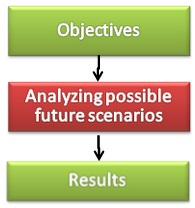
Flowchart:
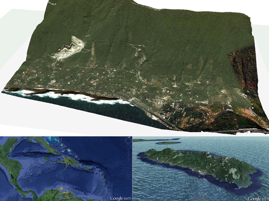
Use case study area description:
The uses cases in this chapter are all dealing with a hypothetical case study of a mountainous slope along the coast of a Caribbean island. It was decided to choose a hypothetical case because of the difficulty in getting the right data for any of the target countries in the the CHARIM project at this stage. This analysis requires local scale hazard intensity maps, detailed element-at-risk maps, vulnerability curves, risk reduction alternatives and future scenarios. Many of these data are still not available for the target countries. Nevertheless we hope that by following the use cases uin this chapter, users get a better idea of the procedure and can eventually also apply it in their onw country, once data is available.
Problems definition and specifications:
The analysis of changes involves the definition of a number of scenarios, which can be seen as trends, on which the users don’t have a direct influence. These can be in terms of:
- Climate change: involving changes in the magnitude-frequency of precipitation extremes and other relevant climatic stimuli (such as evaporation, days with snow cover) and in the occurrence in the time of the year of these extremes (e.g. related to changes in springtime temperature changes).
- Land use change: long term land use changes relate to socio-economic developments that might occur in an area.
- Population change: also related to political and socio-economic developments within a country.
The scenarios are possible developments, and several scenarios are possible for which it will be difficult or impossible to indicate their probability of occurrence.
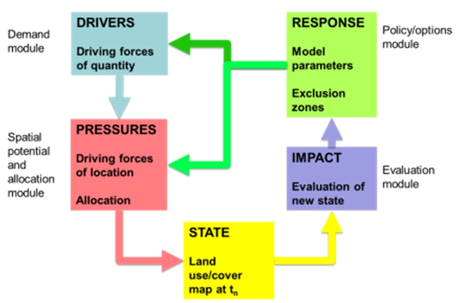
Scenarios of land use /land cover change can be developed using the so-called DPSIR (European Environmental Agency, , which identify the Drivers of change (e.g. economic growth, economic crisis, changes in macro-economic /political constellation, climate change) leading the certain pressures (e.g. increasing demand for land for residential purposes, increasing demand for natural resources), which will alter the existing state, and lead to an impact (e.g. increasing land prices, increasing risk to natural hazards, which may elicit societal response and will feedback on the drivers again (for more information, see : http://www.epa.gov/ged/tutorial/docs/DPSIR_Module_2.pdf)
Data requirements:

Analysis steps:
Step 1: Analyze the input maps
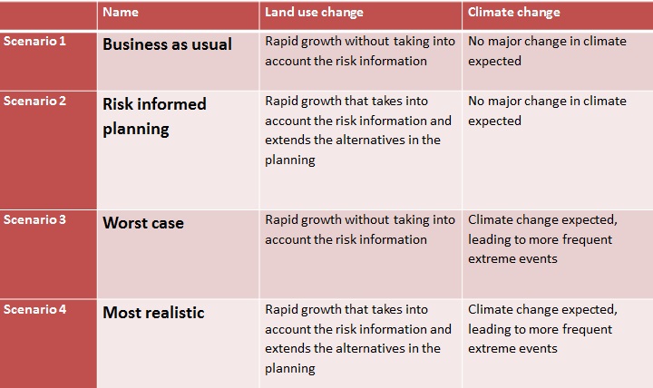
The first step in this analysis is the formulation of possible future future scenarios. This is carried out by external experts on change modelling. In this use case we will consider four possible future scenarios, which are summarized in the table below:
|
|
Name |
Land use change |
Climate change |
|---|---|---|---|
|
Scenario 1 |
Business as usual |
Rapid growth without taking into account the risk information |
No major change in climate expected |
|
Scenario 2 |
Risk informed planning |
Rapid growth that takes into account the risk information and extends the alternatives in the planning |
No major change in climate expected |
|
Scenario 3 |
Worst case |
Rapid growth without taking into account the risk information |
Climate change expected, leading to more frequent extreme events |
|
Scenario 4 |
Most realistic |
Rapid growth that takes into account the risk information and extends the alternatives in the planning |
Climate change expected, leading to more frequent extreme events |
the climate change scenarios in this example are considering the change in return periods of the hazard events, whereas the actual intensity maps are considered to remain the same but the frequency of occurrence is considered to increase. The table below indicates the expected changes in frequency for the four scenarios. Also the range of uncertainty is indicated.
When analyzing future changes we also should define for whicih future year(s) we we analyze the new situation. In this use case we have considered the current situation and fours future years: 2010, 2030 and 2040. this means that we need data for these fours situations. For the changes in frequency the following values are used (obtained from climate change modelling experts):
|
|
New Return Period in Future Year |
||
|---|---|---|---|
|
Old Return Period |
2020 |
2030 |
2040 |
|
20 (± 5) |
17 (± 6) |
14 (± 7) |
11 (± 8) |
|
50 (± 10) |
45 (± 12) |
35 (± 14) |
25 (± 16) |
|
100 (± 20) |
90 (± 23) |
75 (± 26) |
55 (± 30) |
|
200 (± 40) |
180 (± 44) |
150 (± 49) |
110 (± 53) |
The table below indicates which elements-at-risk maps are used for each of the future years. These land use change maps are obtained from experts on landuse change modelling. They are based on certain assumptions (e.g. increase in population, economic growth etc) and also a number of boundary conditions. For example the possible future scenarios 1 and 3 consider that there is no specific emphasis in the growth to avoid hazardous areas, whereas in scenario 2 and 4 the growth tries to avoid the hazardous areas.
|
Possible future scenario: |
Now 2014 |
Elements_at_risk maps : land_parcels |
||
|---|---|---|---|---|
|
2020 |
2030 |
2040 |
||
|
S1 Business as usual |
LP_2014_A0_S0 |
LP_2020_A0_S1 |
LP_2030_A0_S1 |
LP_2040_A0_S1 |
|
S2 Risk informed planning |
LP_2014_A0_S0 |
LP_2020_A0_S2 |
LP_2030_A0_S2 |
LP_2040_A0_S2 |
|
S3 Worst case (Rapid growth + climate change) |
LP_2014_A0_S0 |
LP_2020_A0_S1 |
LP_2030_A0_S1 |
LP_2040_A0_S1 |
|
S4 Climate resilience (informed planning under climate change) |
LP_2014_A0_S0 |
LP_2020_A0_S2 |
LP_2030_A0_S2 |
LP_2040_A0_S2 |
- for scenario 3 and 4 we are using the same element-at-risk maps as for scenario 1 and 2, but we change the frequency of the hazard events (the return periods);
- The actual hazard maps used for the scenarios are the same as those for the alternatives. We do not consider that the intensity will change. Only the return periods of the hazards will change.
Step 2: Analyzing the changes in land use
For analyzing the changes in landuse we are going to calculate the area per land use type for the various land parcel maps of the scenarios, future years and alternatives.
- Create a new table Results_landuse_change, using the domain landuse
- In this table join with the table LP_2014_A0_S0 and aggregate the Area , grouping by Type.
- Check the results in the table Results_landuse_change
We do the land use change analysis in an automate procedure using the script Landuse_change. This script uses three parameters: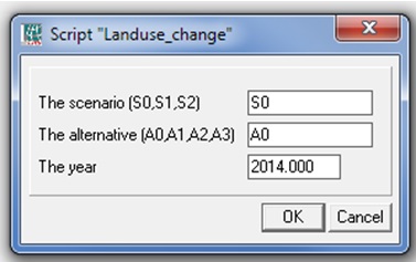
- %1 = The scenario (S0,S1,S2)
- %2 = The alternative (A0,A1,A2,A3)
- %3 = The year
- Open the script and check the statement.
- Run the script for a particular combination of alternative, scenario and year. Best is to do that for the combination marked red in the table on the next page.
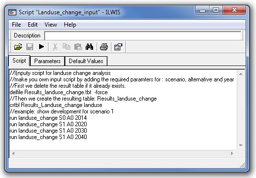
- Adjust the script Landuse_change_input by entering the combinations that you want to analyse.
- The example to the right shows how the Landuse_change_input script could be for analysing the changes in senario 1
- You can run this script by typing on the command line:
Run landuse_change_input
- Present the results in a table (See below), and in a graph in which you show the change in area per land use through time for the different scenarios and alternative combinations.
|
Land use type |
Current situation |
Land use according to scenario 1 and 3 (both have same landuse situation, but different climate change effect) |
Landuse according to scenario 2 and 4 (both have same landuse situation, but different climate change effect) |
||||
|---|---|---|---|---|---|---|---|
|
Hectares 2014 |
2020 |
2030 |
2040 |
2020 |
2030 |
2040 |
|
|
Agricultural_fields |
|
|
|
|
|
|
|
|
Animal_Farm |
|
|
|
|
|
|
|
|
Bare |
|
|
|
|
|
|
|
|
Commercial |
|
|
|
|
|
|
|
|
Cultural_heritage |
|
|
|
|
|
|
|
|
Farm |
|
|
|
|
|
|
|
|
Forest_natural |
|
|
|
|
|
|
|
|
Forest_Planted_protective |
|
|
|
|
|
|
|
|
Grassland |
|
|
|
|
|
|
|
|
Highway |
|
|
|
|
|
|
|
|
Industry |
|
|
|
|
|
|
|
|
Open_slope_soil_removed |
|
|
|
|
|
|
|
|
Orchard |
|
|
|
|
|
|
|
|
Parking_lot |
|
|
|
|
|
|
|
|
Parkland |
|
|
|
|
|
|
|
|
Quarry |
|
|
|
|
|
|
|
|
Residential |
|
|
|
|
|
|
|
|
Shrubs |
|
|
|
|
|
|
|
|
Storage_Basin |
|
|
|
|
|
|
|
|
Toll_area |
|
|
|
|
|
|
|
|
Tourist_resort |
|
|
|
|
|
|
|
|
Vineyard |
|
|
|
|
|
|
|
|
Water_tank |
|
|
|
|
|
|
|
Discuss the results of the land use change given the particular scenario and alternative, and indicate:
- Which developments in land use type do you observe?
- Can you explain these given the scenario / alternative descriptions given earlier?
- What are the main drivers for landuse change?
- Are there un logical development?
Step 3: Analyzing the change in land values
Land values are indicated per land parcel for each of the future scenarios and future years. The land values were estimated based on the land use. The values include the objects on the land and the values represent the replacement costs. In the value estimation the effect of inflation is not considered so that it is better to compare the situation of the different years.
The following table gives the changes in land value per land use type:
Estimated values for scenarios 1 and 3.
|
Land use types |
Value per m2 2014 |
Value per hectare 2014 |
Increase per year |
Value per m2 2020 |
Increase per year |
Value per m2 2030 |
increase per year |
Value per m2 2040 |
|---|---|---|---|---|---|---|---|---|
|
Agricultural_fields |
0.2 |
2000 |
0.01 |
0.2 |
0.01 |
0.2 |
0.01 |
0.3 |
|
Animal_Farm |
300.0 |
3000000 |
0 |
300.0 |
0 |
300.0 |
0 |
300.0 |
|
Bare |
0.0 |
0 |
0 |
0.0 |
0 |
0.0 |
0 |
0.0 |
|
Commercial |
237.0 |
2370000 |
0.01 |
251.6 |
0.01 |
277.9 |
0.01 |
307.0 |
|
Cultural_heritage |
396.0 |
3960000 |
0.02 |
446.0 |
0.02 |
543.6 |
0.02 |
662.7 |
|
Farm |
211.0 |
2110000 |
0 |
211.0 |
0 |
211.0 |
0 |
211.0 |
|
Forest_natural |
11.0 |
110000 |
0 |
11.0 |
0 |
11.0 |
0 |
11.0 |
|
Forest_Planted_protective |
13.0 |
130000 |
0 |
13.0 |
0 |
13.0 |
0 |
13.0 |
|
Grassland |
0.1 |
1000 |
0 |
0.1 |
0 |
0.1 |
0 |
0.1 |
|
Highway |
250.0 |
2500000 |
0 |
250.0 |
0 |
250.0 |
0 |
250.0 |
|
Industry |
300.0 |
3000000 |
0 |
300.0 |
0 |
300.0 |
0 |
300.0 |
|
Open_slope_soil_removed |
0.0 |
0 |
0 |
0.0 |
0 |
0.0 |
0 |
0.0 |
|
Orchard |
2.5 |
25000 |
0.01 |
2.7 |
0.01 |
2.9 |
0.03 |
3.9 |
|
Parking_lot |
150.0 |
1500000 |
0 |
150.0 |
0.01 |
165.7 |
0.03 |
222.7 |
|
Parkland |
15.0 |
150000 |
0 |
15.0 |
0 |
15.0 |
0 |
15.0 |
|
Quarry |
0.1 |
1000 |
0 |
0.1 |
0 |
0.1 |
0 |
0.1 |
|
Residential |
300.0 |
3000000 |
0.01 |
318.5 |
0.02 |
388.2 |
0.03 |
521.7 |
|
Shrubs |
0.0 |
100 |
0 |
0.0 |
0 |
0.0 |
0 |
0.0 |
|
Storage_Basin |
50.0 |
500000 |
0 |
50.0 |
0 |
50.0 |
0 |
50.0 |
|
Toll_area |
350.0 |
3500000 |
0 |
350.0 |
0 |
350.0 |
0 |
350.0 |
|
Tourist_resort |
266.0 |
2660000 |
0.02 |
299.6 |
0.03 |
402.6 |
0.04 |
595.9 |
|
Vineyard |
12.0 |
120000 |
0.03 |
14.3 |
0.04 |
21.2 |
0.06 |
38.0 |
|
Water_tank |
30.0 |
300000 |
0 |
30.0 |
0 |
30.0 |
0 |
30.0 |
Estimated values for scenarios 2 and 4.
|
Land use types |
Value per m2 2014 |
Value per hectare 2014 |
Increase per year |
Value per m2 2020 |
Increase per year |
Value per m2 2030 |
increase per year |
Value per m2 2040 |
|---|---|---|---|---|---|---|---|---|
|
Agricultural_fields |
0.2 |
2000 |
0.01 |
0.2 |
0.01 |
0.2 |
0.01 |
0.3 |
|
Animal_Farm |
300.0 |
3000000 |
0 |
300.0 |
0 |
300.0 |
0 |
300.0 |
|
Bare |
0.0 |
0 |
0 |
0.0 |
0 |
0.0 |
0 |
0.0 |
|
Commercial |
237.0 |
2370000 |
0.04 |
299.9 |
0.06 |
537.0 |
0.07 |
1056.4 |
|
Cultural_heritage |
396.0 |
3960000 |
0.02 |
446.0 |
0.02 |
543.6 |
0.02 |
662.7 |
|
Farm |
211.0 |
2110000 |
0 |
211.0 |
0 |
211.0 |
0 |
211.0 |
|
Forest_natural |
11.0 |
110000 |
0 |
11.0 |
0 |
11.0 |
0 |
11.0 |
|
Forest_Planted_protective |
13.0 |
130000 |
0 |
13.0 |
0 |
13.0 |
0 |
13.0 |
|
Grassland |
0.1 |
1000 |
0 |
0.1 |
0 |
0.1 |
0 |
0.1 |
|
Highway |
250.0 |
2500000 |
0 |
250.0 |
0 |
250.0 |
0 |
250.0 |
|
Industry |
300.0 |
3000000 |
0.04 |
379.6 |
0.06 |
679.8 |
0.07 |
1337.3 |
|
Open_slope_soil_removed |
0.0 |
0 |
0 |
0.0 |
0 |
0.0 |
0 |
0.0 |
|
Orchard |
2.5 |
25000 |
0.01 |
2.7 |
0.01 |
2.9 |
0.03 |
3.9 |
|
Parking_lot |
150.0 |
1500000 |
0 |
150.0 |
0.01 |
165.7 |
0.03 |
222.7 |
|
Parkland |
15.0 |
150000 |
0 |
15.0 |
0 |
15.0 |
0 |
15.0 |
|
Quarry |
0.1 |
1000 |
0 |
0.1 |
0 |
0.1 |
0 |
0.1 |
|
Residential |
300.0 |
3000000 |
0.05 |
402.0 |
0.07 |
790.9 |
0.1 |
2051.3 |
|
Shrubs |
0.0 |
100 |
0 |
0.0 |
0 |
0.0 |
0 |
0.0 |
|
Storage_Basin |
50.0 |
500000 |
0 |
50.0 |
0 |
50.0 |
0 |
50.0 |
|
Toll_area |
350.0 |
3500000 |
0 |
350.0 |
0 |
350.0 |
0 |
350.0 |
|
Tourist_resort |
266.0 |
2660000 |
0.04 |
336.6 |
0.05 |
548.2 |
0.06 |
981.8 |
|
Vineyard |
12.0 |
120000 |
0.03 |
14.3 |
0.04 |
21.2 |
0.06 |
38.0 |
Land value change can be analysed in different ways. You could do this for administrative units, for land use types, or for the entire area. The easiest method is to do this for the whole area. You can directly get the total land values from the attribute tables.
 Open the table LP_2014_A0_S0. Check whether the statistics pane is visible. You can read the total value for this combination.
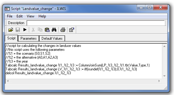
- For the analysis of land value changes we use a script: Landvalue_change See right)
- This script has the following variables:
- %1 = the scenario (S0,S1,S2)
- %2 = the alternative (A0,A1,A2,A3)
- %3 = the year
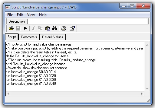 The actual analysis of land value changes is done using an input script: Landvalue_change_input. And example of this is given here for analysing the land value changes for scenario 1.
 - Run this script by typing: Run Landvalue_change_input
- Adjust the Landvalue_change_input script so that also the other scenarios are included. Do this by copying the content in a text editor and changing them.
- Then run the input script and after the calculation is done, investigate the results and write them in a table like the one below.
Note that the results for scenario 1 and 3 and for scenario 2 and 4 are the same as the land use for scenario 3 is the same as for scenario 1 and the ones from scenario 4 the same as scenario 2 (only the frequency of hazard events changes due to climate change effects).
Present the results in a table, and in a graph in which you show the change in area per land use through time for the different scenarios and alternative combinations.
|
Scenario: Possible Future trends |
Current situation |
Future years |
||
|---|---|---|---|---|
|
2020 |
2030 |
2040 |
||
|
S1 Business as usual |
|
|
|
|
|
S2 Risk informed planning |
|
|
|
|
|
S3 Worst case (Rapid growth + climate change) |
|
|
|
|
|
S4 Climate resilience (informed planning under climate change) |
|
|
|
|
Step 3: Analyzing the changes in population
Also population densities and number of people are indicated per land parcel for each of the future scenarios and future years. The population data were estimated based on the land use. The number of people are considered maximum values, and not specific population scenarios (e.g. daytime night-time, summer / winter etc.) have been considered. The tables below show the data on the basis of which the estimations were made:
Scenario 1 and 3: Population data
|
Land use type |
People per m2 2014 |
People per hectare 2014 |
Increase per year |
People per m2 2020 |
Increase per year |
People per m2 2030 |
increase per year |
People per m2 2040 |
People per hectare 2014 |
|---|---|---|---|---|---|---|---|---|---|
|
Agricultural_fields |
0.00001 |
1 |
0 |
0.00001 |
0 |
0.00001 |
0 |
0.00001 |
1 |
|
Animal_Farm |
0.00005 |
5 |
0 |
0.00005 |
0 |
0.00005 |
0 |
0.00005 |
5 |
|
Bare |
0.00000 |
0 |
0 |
0.00000 |
0 |
0.00000 |
0 |
0.00000 |
0 |
|
Commercial |
0.00500 |
500 |
0 |
0.00500 |
0 |
0.00500 |
0 |
0.00500 |
500 |
|
Cultural_heritage |
0.00100 |
100 |
0 |
0.00100 |
0 |
0.00100 |
0 |
0.00100 |
100 |
|
Farm |
0.00005 |
5 |
0 |
0.00005 |
0 |
0.00005 |
0 |
0.00005 |
5 |
|
Forest_natural |
0.00001 |
1 |
0 |
0.00001 |
0 |
0.00001 |
0 |
0.00001 |
1 |
|
Forest_Planted_protective |
0.00002 |
2 |
0 |
0.00002 |
0 |
0.00002 |
0 |
0.00002 |
2 |
|
Grassland |
0.00000 |
0.1 |
0 |
0.00000 |
0 |
0.00000 |
0 |
0.00000 |
0 |
|
Highway |
0.00500 |
500 |
0 |
0.00500 |
0 |
0.00500 |
0 |
0.00500 |
500 |
|
Industry |
0.00100 |
100 |
0 |
0.00100 |
0 |
0.00100 |
0 |
0.00100 |
100 |
|
Open_slope_soil_removed |
0.00000 |
0 |
0 |
0.00000 |
0 |
0.00000 |
0 |
0.00000 |
0 |
|
Orchard |
0.00003 |
2.5 |
0 |
0.00003 |
0 |
0.00003 |
0 |
0.00003 |
3 |
|
Parking_lot |
0.00100 |
100 |
0 |
0.00100 |
0 |
0.00100 |
0 |
0.00100 |
100 |
|
Parkland |
0.00020 |
20 |
0 |
0.00020 |
0 |
0.00020 |
0 |
0.00020 |
20 |
|
Quarry |
0.00005 |
5 |
0 |
0.00005 |
0 |
0.00005 |
0 |
0.00005 |
5 |
|
Residential |
0.00040 |
40 |
0.01 |
0.00042 |
0.02 |
0.00052 |
0.03 |
0.00070 |
70 |
|
Shrubs |
0.00000 |
0 |
0 |
0.00000 |
0 |
0.00000 |
0 |
0.00000 |
0 |
|
Storage_Basin |
0.00000 |
0 |
0 |
0.00000 |
0 |
0.00000 |
0 |
0.00000 |
0 |
|
Toll_area |
0.00500 |
500 |
0 |
0.00500 |
0 |
0.00500 |
0 |
0.00500 |
500 |
|
Tourist_resort |
0.00150 |
150 |
0 |
0.00150 |
0 |
0.00150 |
0 |
0.00150 |
150 |
|
Vineyard |
0.00020 |
20 |
0 |
0.00020 |
0 |
0.00020 |
0 |
0.00020 |
20 |
|
Water_tank |
0.00000 |
0 |
0 |
0.00000 |
0 |
0.00000 |
0 |
0.00000 |
0 |
Scenario 2 and 4: Population data
|
Land use type |
People per m2 2014 |
People per hectare 2014 |
Increase per year |
People per m2 2020 |
Increase per year |
People per m2 2030 |
increase per year |
People per m2 2040 |
People per hectare 2014 |
|---|---|---|---|---|---|---|---|---|---|
|
Agricultural_fields |
0.00001 |
1 |
0 |
0.00001 |
0 |
0.00001 |
0 |
0.00001 |
1 |
|
Animal_Farm |
0.00005 |
5 |
0 |
0.00005 |
0 |
0.00005 |
0 |
0.00005 |
5 |
|
Bare |
0.00000 |
0 |
0 |
0.00000 |
0 |
0.00000 |
0 |
0.00000 |
0 |
|
Commercial |
0.00500 |
500 |
0 |
0.00500 |
0 |
0.00500 |
0 |
0.00500 |
500 |
|
Cultural_heritage |
0.00100 |
100 |
0 |
0.00100 |
0 |
0.00100 |
0 |
0.00100 |
100 |
|
Farm |
0.00005 |
5 |
0 |
0.00005 |
0 |
0.00005 |
0 |
0.00005 |
5 |
|
Forest_natural |
0.00001 |
1 |
0 |
0.00001 |
0 |
0.00001 |
0 |
0.00001 |
1 |
|
Forest_Planted_protective |
0.00002 |
2 |
0 |
0.00002 |
0 |
0.00002 |
0 |
0.00002 |
2 |
|
Grassland |
0.00000 |
0.1 |
0 |
0.00000 |
0 |
0.00000 |
0 |
0.00000 |
0 |
|
Highway |
0.00500 |
500 |
0 |
0.00500 |
0 |
0.00500 |
0 |
0.00500 |
500 |
|
Industry |
0.00100 |
100 |
0 |
0.00100 |
0 |
0.00100 |
0 |
0.00100 |
100 |
|
Open_slope_soil_removed |
0.00000 |
0 |
0 |
0.00000 |
0 |
0.00000 |
0 |
0.00000 |
0 |
|
Orchard |
0.00003 |
2.5 |
0 |
0.00003 |
0 |
0.00003 |
0 |
0.00003 |
3 |
|
Parking_lot |
0.00100 |
100 |
0 |
0.00100 |
0 |
0.00100 |
0 |
0.00100 |
100 |
|
Parkland |
0.00020 |
20 |
0 |
0.00020 |
0 |
0.00020 |
0 |
0.00020 |
20 |
|
Quarry |
0.00005 |
5 |
0 |
0.00005 |
0 |
0.00005 |
0 |
0.00005 |
5 |
|
Residential |
0.00040 |
40 |
0.05 |
0.00054 |
0.1 |
0.00139 |
0.1 |
0.00361 |
361 |
|
Shrubs |
0.00000 |
0 |
0 |
0.00000 |
0 |
0.00000 |
0 |
0.00000 |
0 |
|
Storage_Basin |
0.00000 |
0 |
0 |
0.00000 |
0 |
0.00000 |
0 |
0.00000 |
0 |
|
Toll_area |
0.00500 |
500 |
0 |
0.00500 |
0 |
0.00500 |
0 |
0.00500 |
500 |
|
Tourist_resort |
0.00150 |
150 |
0 |
0.00150 |
0 |
0.00150 |
0 |
0.00150 |
150 |
|
Vineyard |
0.00020 |
20 |
0 |
0.00020 |
0 |
0.00020 |
0 |
0.00020 |
20 |
|
Water_tank |
0.00000 |
0 |
0 |
0.00000 |
0 |
0.00000 |
0 |
0.00000 |
0 |
Population change can be analysed in different ways. You could do this for administrative units, for land use types, or for the entire area. The easiest method is to do this for the whole area. You can directly get the total population values from the attribute tables.
 Open the table LP_2014_A0_S0. Check whether the statistics pane is visible. You can read the population information for this combination.
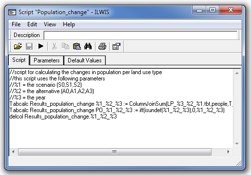
 - For the analysis of land value changes we use a script: Population_change See right)
- This script has the following variables:
- %1 = the scenario (S0,S1,S2)
- %2 = the alternative (A0,A1,A2,A3)
- %3 = the year
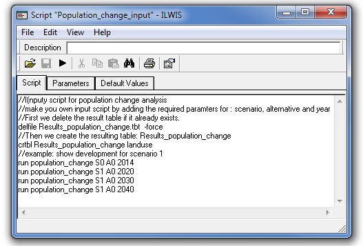 The actual analysis of population changes is done using an input script: Population_change_input. An example of this is given here for analysing the population changes for scenario 1.
- Run this script by typing:
- Run Population_change_input
- Adjust the Population_change_input script so that also the other scenarios are included. Do this by copying the content in a text editor and changing them.
- Then run the input script and after the calculation is done, investigate the results and write them in a table like the one below.
- Note that the results for scenario 1 and 3 and for scenario 2 and 4 are the same as the land use for scenario 3 is the same as for scenario 1 and the ones from scenario 4 the same as scenario 2 (only the frequency of hazard events changes due to climate change effects).
|
Scenario: Possible Future trends |
Current situation |
Future years |
||
|---|---|---|---|---|
|
2020 |
2030 |
2040 |
||
|
S1 Business as usual |
|
|
|
|
|
S2 Risk informed planning |
|
|
|
|
|
S3 Worst case (Rapid growth + climate change) |
|
|
|
|
|
S4 Climate resilience (informed planning under climate change) |
|
|
|
|
Step 4: Analyzing the changes in risk
Similarly as the analysis which was done for the current risk and for the evaluation of the best risk reduction alternative, we are doing this analysis in two steps:
- Loss analysis for each individual combination of hazard set (for a given date, hazard type and return
- Period) and elements-at-risk (the land parcel map for the given scenario and future year).
- Risk analysis by combining the loss results for different hazards and return periods.
Loss analysis.
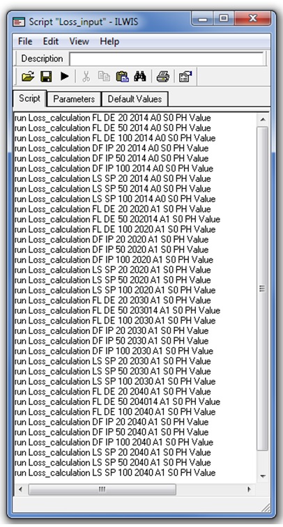
You can also analyse the changes in risk for the different scenarios. This will take more time, but you can use the script Loss_calculation for that
- Adapt the script Loss_input and add the specific combinations of scenarios, and future years
- The best is to copy the text in a text editor and adjust the parameters like the future year and the scenario number.
- The example on the right side show the situation for the scenario 1 for the current situation and for 3 future years: 2020, 2030 and 2040.
- After generating the input script, you can run it and one by one the actual loss estimation script (Loss_calculation) is calculated, everytime with another set of input data.
- Each time the results of the analysis are written in three tables with the results: Results_LP (for each landparcel the results are stored), Result_Admin_Units (results aggregated per administrative units) and Results_Total (Aggregated values for the entire area).
- The calculation might take quite some time (probably at least one hour, since many calculations have to be made)
When the calculation is completed, check the results from the tables indicated above.
Risk analysis
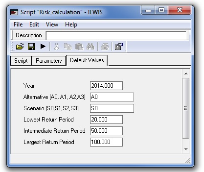
The risk analysis which was done using a scrip Risk_calculation (see previous exercises) can now also be done for the different scenarios. Remember that the script has the following vairables:
%1 = Year
%2 = Alternative
%3 = Scenario
%4 = First return period
%5 = Second return period
%6 = Third return period
We assume that flooding, landslides and debrisflows are depending on the same trigger, so we take the maximum losses for a given area from one of the three hazards. We assume that if a triggering events occurs it may trigger either landslides, flashfloods or debrisflows, and the area affected by one would lead to a certain amount of losses. If another event also happens it will not cause twice the same damage.
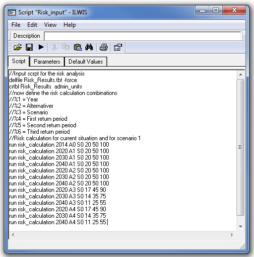 The input data for the risk analysis is handled through the scrip Risk_calculation_input. For running the scenarios 1 to 4 the following information should be available:
Note that we first calculate the current risk, and then calculate the risk for the four different scenarios.
- Scenario 1 and 2 use the same return periods as the current situation, as both of these scenarios only consider land use changes, and the losses for these were calculated in the loss calculation. There is no climate change effect considered, so therefore we use the same return periods as for the current situation.
- However for scenarios 2 and 4 we adjust the return periods based on the change in expected frequencies that are coming from the climate change analysis. The table with these values was presented in the beginning in the section dealing with the input data.
- Adapt the Risk_calculation_input script so that it represents the same situation as the one shown above.
- Then run the script by typing on the command line:
Run Risk_calculation_input
- Calculate the annualized risk for the combinations indicated and put these in the table
- Present the results in a table, and in a graph in which you show the change in area per land use through time for the different scenarios and alternative combinations.
|
Scenario: Possible Future trends |
Alternative: risk reduction options |
Future years |
||
|---|---|---|---|---|
|
2020 |
2030 |
2040 |
||
|
S1 Business as usual |
A0 (no risk reduction) |
|
|
|
|
S2 Risk informed planning |
A0 (no risk reduction) |
|
|
|
|
S3 Worst case (Rapid growth + climate change) |
A0 (no risk reduction) |
|
|
|
|
S4 Climate resilience (informed planning under climate change) |
A0 (no risk reduction) |
|
|
|
Step 5: summary
After analysing the land use change, land value change and population change, you can now give a more thorough evaluation of the changes and the drivers.
- Analyse the changes in land use for the different scenarios in a number of future years (2020, 2030 and 2040) and explain the trends and possible drivers;
- Analyse the changes in economic values for the different scenarios in a number of future years (2020, 2030 and 2040)
- Analyse the changes in population for the different scenarios in a number of future years (2020, 2030 and 2040)
- Analyse the changes in risk for the for the different scenarios in a number of future years (2020, 2030 and 2040)
Results:
This section will show the results for the analysis:
Analysis of landuse changes
The table below shows the results of the land use change for the different scenarios and future years.
|
|
|
Land use according to scenario 1 and 3 (both have same landuse situation, but different climate change effect) |
Landuse according to scenario 2 and 4 (both have same landuse situation, but different climate change effect) |
||||
|---|---|---|---|---|---|---|---|
|
2014 |
2020 |
2030 |
2040 |
2020 |
2030 |
2040 |
|
|
Agricultural_fields |
85205 |
54342 |
0 |
0 |
24435 |
4301 |
4301 |
|
Animal_Farm |
9639 |
9639 |
4301 |
0 |
9639 |
9639 |
9639 |
|
Bare |
31354 |
2785 |
2042 |
0 |
1314 |
743 |
743 |
|
Commercial |
18772 |
61989 |
90410 |
151300 |
25144 |
36918 |
42070 |
|
Cultural_heritage |
4289 |
4289 |
4831 |
4831 |
4289 |
4289 |
4289 |
|
Farm |
117829 |
99823 |
67847 |
42893 |
110705 |
98036 |
91086 |
|
Forest_natural |
2687779 |
2674466 |
2667449 |
2685162 |
2678630 |
2671613 |
2690797 |
|
Forest_Planted_protective |
309301 |
304793 |
332458 |
332458 |
362170 |
362170 |
362170 |
|
Grassland |
35890 |
39970 |
16558 |
16558 |
39645 |
20461 |
16558 |
|
Highway |
55811 |
55811 |
55811 |
55811 |
55811 |
55811 |
55811 |
|
Industry |
44465 |
55188 |
63389 |
76736 |
44465 |
39750 |
39750 |
|
Orchard |
665137 |
618232 |
517087 |
357962 |
632086 |
582562 |
560447 |
|
Parking_lot |
1166 |
5063 |
13858 |
17281 |
1166 |
1622 |
1622 |
|
Parkland |
18556 |
33679 |
70149 |
74450 |
39868 |
58919 |
54722 |
|
Quarry |
115095 |
128408 |
140650 |
140650 |
128408 |
140650 |
140650 |
|
Residential |
125954 |
194402 |
327795 |
465811 |
195936 |
279402 |
335971 |
|
Shrubs |
90855 |
69325 |
63607 |
43445 |
35471 |
31374 |
9569 |
|
Toll_area |
13960 |
13960 |
13960 |
13960 |
13960 |
13960 |
13960 |
|
Tourist_resort |
22934 |
47884 |
64110 |
76705 |
30619 |
49581 |
49581 |
|
Vineyard |
293786 |
273729 |
231465 |
191764 |
314016 |
285976 |
264041 |
|
Water_tank |
2813 |
2813 |
2813 |
2813 |
2813 |
2813 |
2813 |
You can also calculate the percentage change with respect to the current situation.
Analysis of changes in values
The following table shows the results of the analysis of changes in land value:
|
|
|
Land use according to scenario 1 and 3 (both have same landuse situation, but different climate change effect) |
Landuse according to scenario 2 and 4 (both have same landuse situation, but different climate change effect) |
||||
|---|---|---|---|---|---|---|---|
|
2014 |
2020 |
2030 |
2040 |
2020 |
2030 |
2040 |
|
|
Agricultural_fields |
1.15E+04 |
5.66E+03 |
0.00E+00 |
0.00E+00 |
1.30E+04 |
2.52E+03 |
2.79E+03 |
|
Animal_Farm |
6.27E+06 |
6.27E+06 |
1.29E+06 |
0.00E+00 |
4.82E+04 |
4.82E+04 |
4.82E+04 |
|
Bare |
0.00E+00 |
0.00E+00 |
0.00E+00 |
0.00E+00 |
0.00E+00 |
0.00E+00 |
0.00E+00 |
|
Commercial |
4.30E+06 |
1.54E+07 |
2.50E+07 |
4.63E+07 |
7.35E+06 |
1.95E+07 |
4.38E+07 |
|
Cultural_heritage |
1.52E+06 |
1.71E+06 |
2.38E+06 |
2.90E+06 |
6.87E+05 |
8.38E+05 |
1.02E+06 |
|
Farm |
1.82E+07 |
1.61E+07 |
1.21E+07 |
7.57E+06 |
1.66E+07 |
1.44E+07 |
1.39E+07 |
|
Forest_natural |
2.95E+07 |
2.93E+07 |
2.93E+07 |
2.95E+07 |
1.38E+06 |
1.43E+06 |
1.64E+06 |
|
Forest_Planted_protective |
4.02E+06 |
3.96E+06 |
4.32E+06 |
4.32E+06 |
9.90E+05 |
9.90E+05 |
9.90E+05 |
|
Grassland |
1.55E+05 |
1.55E+05 |
1.53E+05 |
1.53E+05 |
1.66E+05 |
1.64E+05 |
1.64E+05 |
|
Highway |
0.00E+00 |
0.00E+00 |
0.00E+00 |
0.00E+00 |
0.00E+00 |
0.00E+00 |
0.00E+00 |
|
Industry |
9.76E+06 |
1.30E+07 |
1.54E+07 |
1.94E+07 |
6.84E+06 |
1.10E+07 |
2.16E+07 |
|
Open_slope_soil_removed |
0.00E+00 |
0.00E+00 |
0.00E+00 |
0.00E+00 |
0.00E+00 |
0.00E+00 |
0.00E+00 |
|
Orchard |
2.22E+06 |
2.03E+06 |
1.47E+06 |
1.41E+06 |
1.34E+06 |
1.39E+06 |
1.81E+06 |
|
Parking_lot |
1.75E+05 |
7.59E+05 |
2.30E+06 |
3.85E+06 |
2.33E+03 |
7.81E+04 |
1.05E+05 |
|
Parkland |
1.59E+05 |
3.86E+05 |
9.33E+05 |
9.97E+05 |
3.27E+05 |
6.13E+05 |
5.50E+05 |
|
Quarry |
2.54E+05 |
2.56E+05 |
2.57E+05 |
2.57E+05 |
2.56E+05 |
2.57E+05 |
2.57E+05 |
|
Residential |
2.32E+07 |
4.64E+07 |
1.08E+08 |
2.18E+08 |
5.89E+07 |
1.82E+08 |
5.88E+08 |
|
Shrubs |
0.00E+00 |
0.00E+00 |
0.00E+00 |
0.00E+00 |
0.00E+00 |
0.00E+00 |
0.00E+00 |
|
Storage_Basin |
0.00E+00 |
0.00E+00 |
0.00E+00 |
0.00E+00 |
0.00E+00 |
0.00E+00 |
0.00E+00 |
|
Toll_area |
4.89E+06 |
4.89E+06 |
4.89E+06 |
4.89E+06 |
3.49E+04 |
3.49E+04 |
3.49E+04 |
|
Tourist_resort |
4.70E+06 |
1.28E+07 |
2.56E+07 |
4.54E+07 |
8.60E+06 |
2.44E+07 |
4.37E+07 |
|
Vineyard |
3.53E+06 |
3.92E+06 |
4.91E+06 |
7.28E+06 |
8.16E+05 |
1.18E+06 |
2.09E+06 |
|
Water_tank |
8.44E+04 |
8.44E+04 |
8.44E+04 |
8.44E+04 |
9.85E+05 |
9.85E+05 |
9.85E+05 |
|
Total value |
1.13E+08 |
1.57E+08 |
2.39E+08 |
3.92E+08 |
1.05E+08 |
2.59E+08 |
7.20E+08 |
Analysis of changes in population
The following table shows the results of the analysis of population
|
|
|
Land use according to scenario 1 and 3 (both have same landuse situation, but different climate change effect) |
Landuse according to scenario 2 and 4 (both have same landuse situation, but different climate change effect) |
||||
|---|---|---|---|---|---|---|---|
|
2014 |
2020 |
2030 |
2040 |
2020 |
2030 |
2040 |
|
|
Agricultural_fields |
0 |
0 |
0 |
0 |
2 |
0 |
0 |
|
Animal_Farm |
0 |
0 |
0 |
0 |
2 |
2 |
2 |
|
Bare |
0 |
0 |
0 |
0 |
0 |
0 |
0 |
|
Commercial |
119 |
335 |
477 |
781 |
151 |
210 |
235 |
|
Cultural_heritage |
15 |
15 |
16 |
16 |
13 |
13 |
13 |
|
Farm |
305 |
273 |
168 |
89 |
238 |
206 |
199 |
|
Forest_natural |
22 |
22 |
22 |
22 |
22 |
22 |
22 |
|
Forest_Planted_protective |
6 |
6 |
7 |
7 |
7 |
7 |
7 |
|
Grassland |
2 |
2 |
2 |
2 |
16 |
16 |
16 |
|
Highway |
0 |
0 |
0 |
0 |
0 |
0 |
0 |
|
Industry |
110 |
121 |
129 |
143 |
111 |
95 |
95 |
|
Open_slope_soil_removed |
0 |
0 |
0 |
0 |
0 |
0 |
0 |
|
Orchard |
27 |
24 |
1 |
1 |
16 |
6 |
6 |
|
Parking_lot |
1 |
5 |
14 |
17 |
2 |
2 |
2 |
|
Parkland |
2 |
5 |
12 |
13 |
6 |
10 |
9 |
|
Quarry |
5 |
6 |
7 |
7 |
6 |
7 |
7 |
|
Residential |
553 |
604 |
815 |
1180 |
779 |
2135 |
5757 |
|
Shrubs |
0 |
0 |
0 |
0 |
0 |
0 |
0 |
|
Storage_Basin |
0 |
0 |
0 |
0 |
0 |
0 |
0 |
|
Toll_area |
70 |
70 |
70 |
70 |
42 |
42 |
42 |
|
Tourist_resort |
142 |
180 |
206 |
224 |
158 |
186 |
186 |
|
Vineyard |
60 |
57 |
48 |
39 |
64 |
58 |
54 |
|
Water_tank |
0 |
0 |
0 |
0 |
0 |
0 |
0 |
|
Total population |
1439 |
1725 |
1994 |
2611 |
1635 |
3017 |
6652 |
Analysis of changes in risk
The following table shows the changes in risk.
Conclusions:
The use case allows users to evaluate the effect of possible future scenarios on the changes in risk. These scenarios can be related top climate change and/or land use change. The scenarios themselves need to be generated by consultants with knowledge on the translation of future trends in triggering events (e.g. as a results of climate change) for the change of return periods. Also experts are needed for analyzing the possible changes for land use under possible future scenarios. these scenarios can also be different land use planning scenarios.
- The analysis is complicated, and requires a lot of input data. The most important sources of uncertainty in this analysis are:
- the analysis of the current hazards. This refers to analyzing intensity maps for different return periods.
- the collection of elements-at-risk data, with characterization of value information and population information
- the link between elements-at-risk and hazards through vulnerability curves.
- the formulation of future climate change scenarios and the effect of these on changing return periods.
- the formulation of possible future land use change scenarios. In this use case we did this using land use. Doing this for other elements-at-risk such as building footprints is much more complicated still.
Nevertheless the use case allows you to analyze what are the possible consequences of future scenarios, which should be an important component in the planning process.