6.2 Spatial Multi-Criteria Evaluation

Authors: D. Alkema, and L.G.J. Boerboom, S. Ferlisi and L. Cascini

Keywords: Spatial Multi Criteria Evaluation, Multi-Hazard Risk Assessment, Landslides, Floods

Introduction

Spatial Multi-Criteria Evaluation (SMCE) represents a relatively new concept for the qualitative analysis and zoning of the risk due to a number of natural hazards, e.g. landslides, floods or earthquakes (Rashed and Weeks 2003, Alkema 2007, Castellanos 2008, Dang 2011). It is a useful complementary method to the existing approaches for qualitative and quantitative risk analysis and zoning. Moreover, SMCE can facilitate participatory processes aimed at choosing sustainable risk mitigation measures and can support decision makers, who are faced with making evaluations of projects or policies based on multiple criteria, in identifying - for instance -  priority areas for actions to reduce risk.

This chapter gives an overview of the main issues concerning SMCE and its usefulness for decision-making in an area exposed to multiple hazards. It describes the procedure for Spatial Multi-Criteria Evaluation by applying SMCE to a hypothetical situation on one of the Caribbean islands. A more in-depth approach is described in use cases 4.1 - 4.6. In the discussion some strengths and weaknesses of SMCE are discussed.

Spatial Multi-Criteria Evaluation (SMCE)

Spatial Multi-Criteria Evaluation can be thought of as a process that combines and transforms a number of geographical data (input) into a resultant decision (output) - see Figure 1 (Malczewski 1999). The result is an aggregation of multi-dimensional information into a single parameter output map: the decision. This process includes, apart from geographical data, also the decision maker's preferences and the manipulation of the data and preferences according to specified decision rules. SMCE is a decision support tool that forces the assessors (e.g. teams of experts and stakeholders) to structure their problem and outline their information requirements. Initially such systems were developed for complex business decisions but in the last 20 years they have  been applied to spatial problems as well, see e.g. Carver (1991), Chen et al. (2001), Sharifi et al. (2002), Pfeffer (2003), Zucca (2005) and Malczewski (2006).

  

 Figure 1. Spatial multi criteria evaluation (after Malczewski 1999).

 

SMCE for decision-making

Rational decision-making requires a careful analysis of the decision problem. In case of complex problems a frequently used approach is to decompose the problem into smaller, understandable parts. This approach is called Analytical Hierarchy Process (AHP) which is described by e.g. Saaty (1980). The smaller, understandable parts are called the evaluation criteria and these can be further decomposed into objectives and attributes (Saaty 1980, Malczewski 1999, Pfeffer 2003). An objective conveys a desired state that an individual or group would like to achieve, while an attribute is used to characterise an objective. The decomposition of a problem can be structured in a so-called criteria tree - see Figure 2. Attributes can be quantified by indicator maps that provide the input for the analysis wih parameter values (e.g. flood depth maps).

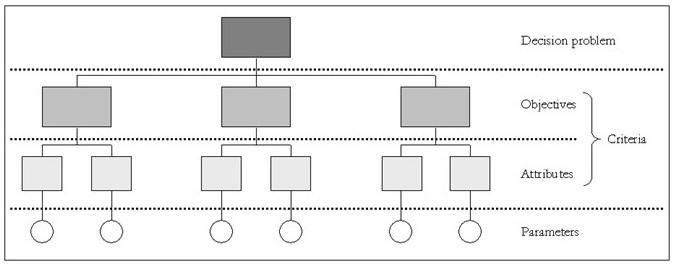
 Figure 2. The SMCE criteria tree to decompose a decision problem into objectives, attributes and parameters. In principal there is no restriction to the number of hierarchical levels of objectives and attributes.

 

SMCE: Discrete and continuous evaluation

Some authors, e.g. Beinat (1997) make a distinction between discrete and continuous evaluations. Discrete evaluations tackle choice problems in which alternatives are selected from a discrete (and limited) set of alternatives to identify the best option. Continuous evaluations are more suitable for design problems (Beinat, 1997) and to identify priority areas. Some authors define the latter type of evaluation as multi-objective decision-making (e.g., Hwang and Masud, 1979; Malczewski, 1999). The evaluation of risk, which does not evaluate a set of alternatives, is a typical example of continuous evaluation. 

SMCE: A multi-stakeholder tool

Spatial multi-criteria evaluation is a suitable tool to structure discussions about a decision problem where multiple assessors or stakeholders are involved. The underlying proposition is if all stakeholders reach agreement on the decision problem, the set of criteria and parameters, and on the aggregation procedure, they are likely to agree on the outcome. Hence SMCE adds to the decision-making process in that it identifies agreements and disagreements between the stakeholders, that it brings understanding, supports learning-by-doing and that it reveals areas where further thinking is necessary (Beinat 1997). Furthermore, SMCE supports the solution of a decision problem by analysing its robustness with respect to uncertainty (Geneletti 2002, Ullman 2006).

Rothenberg (1975) makes a distinction between a team assessment and a coalition assessment. A team is defined as a group of people with a mutually consistent set of preferences. Even though a team may consist of many people, they seem to act as a single entity because they have a common vision on the decision problem and the criteria evaluation to address that problem. A coalition on the other hand can be defined as a group of people who compromise their partly similar, partly divergent outlooks. Coalition partners can agree on the decision problem and on the structure of the criteria tree but may disagree on the relative importance of the evaluation criteria. The consequence of these different opinions is that it usually necessitates multiple analyses to accommodate the various preferences of the coalition participants, whereas a single analysis is often possible for team members (Malczewski, 1999). 

Steps in SMCE

In the transformation process of the parameter maps into a decision, four consecutive steps have to be taken by the assessment team: 1) structuring the decision problem; 2) the standardisation of or value judgment about the parameter maps according to explicitly formulated criteria; 3) the establishment of the importance of each individual criterion with respect to other criteria and the decision problem; and 4) the aggregation procedure. An additional sensitivity analysis can be included to test the robustness of the outcome. 

1 Structuring the criteria tree: In essence this means that a big decision problem is decomposed into smaller understandable parts. The assessment team must construct a criteria tree in such a manner that all the evaluation criteria are incorporated. If agreement has been reached how to solve each of these smaller parts, the big problem can be solved too. 

2 Standardisation: Each parameter has its own physical units and scale of measurement which makes that the values cannot be directly compared with each other. This would result in physically meaningless numbers and make them dependent on the scale of measurement. Therefore standardisation is required to transform the parameter values into scores on an equal, dimensionless scale e.g. between 0 and 1. The transformation - or value assessment (Geneletti 2002) - is done with a value function and transforms the parameter values of each parameter map into scores on an equal, dimensionless scale - often between 0 and 1. The value function is a mathematical relationship that is defined by, for example, laws, research findings, or by stakeholders and can include human judgements and knowledge but also bias and perception. The value function explicitly links the factual information in the parameter maps to the corresponding parameter scores - see figure 3. In practice standardization should always be a group process so that all views of the different stakeholders are incorporated and that they all agree on the value functions. Beinat (1997) gives a good overview of the difficulties that may arise in defining value functions and shows examples of how these can be mitigated - or at least be handled.

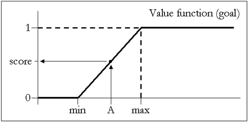
Figure 3. Example of a value function (type goal): on the horizontal axis are all possible values of a certain parameter map. Values below the lower threshold (min) get a corresponding standardized score of 0, values above the higher threshold (max) get a corresponding score of 1, where 0 means no attainment of a criterion whereas 1 means full attainement of the criterion.

 

3 Prioritisation: During the prioritisation step weights are assigned to the criteria to reflect the importance of each criterion relatively to the other criteria under consideration (Malczewski 1999). The assignment of the weights is the second crucial step that, like the standardization, is a group process in which the assessors will have to reach agreement. Various methods have been developed to guide the assessors through the prioritisation process. Among these are the following (Malczewski, 1999):

Ranking methods in which the assessor ranks the criteria in order of preference. The numerical weights are then assigned as function of the rank;
Rating methods in which the assessor assigns weights on a predetermined scale to each criterion using a predefined procedure. The numerical weights are then assigned by normalisation (dividing each weight by the sum of all weights);

Pair-wise comparison method in which the assessor compares each possible pair of criteria and rates one relative to the other on a scale from equal importance to extremely more important. Comparison of all possible pairs results in a so-called ratio-matrix. The numerical weights are determined by normalizing the eigenvector associated with the maximum eigenvalue of the ratio matrix (Saaty, 1980). 

4 Aggregation: After the standardisation of each parameter and prioritisation of the parameters relatively to one and another, the maps must be combined in a decision model. This is called the aggregation step (Geneletti 2002). Because the results of the value functions are all on a scale from 0 to 1 and because the sum of the normalised weights equals 1, the result is a dimensionless scalar map with scores between 0 and 1. The result is sometimes called "the decision" or "composite index map'. Scores close to 0 identify areas where the criteria are absolutely disadvantageous and scores close to 1 indicate areas that meet the criteria perfectly. Figure 4 gives a summary of the procedure.

 

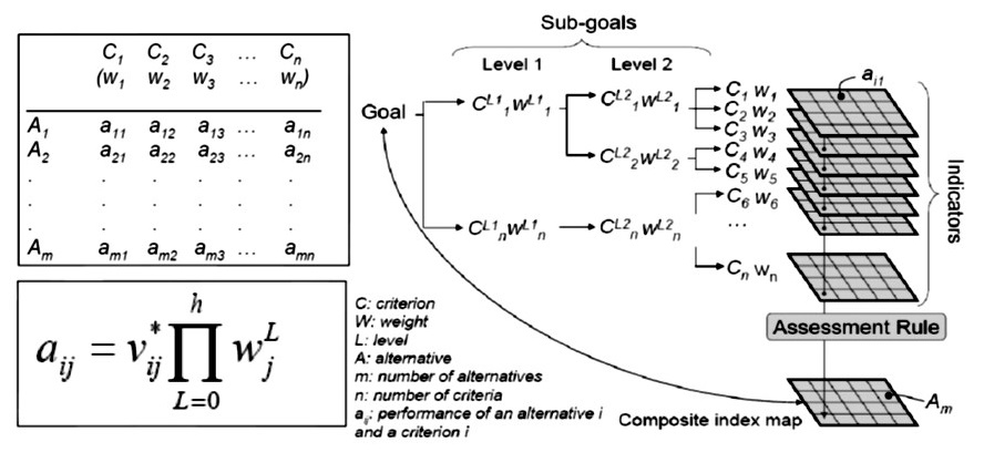
Figure 4. Schematic procedure for spatial multi-criteria evaluation based on the analytical hierarchical process (Castellanos 2008). 

The most widely used aggregation method is the weighted linear combination, also called simple additive weighting or scoring method. This method is based on the concept of weighted average (Malczewski, 1999). In its simplest form a decision could be defined as: 

F(x) = Sn(Wk (fk(x)))

Where:

F(x)        = the outcome (the decision) as a result of n criteria.

Wk          = the normalised non-negative weight of the kth criterion.

fk(x)       = the value function of the kth criterion.

Because the results of the value functions are on a scale from 0 to 1 and because the sum of the normalised weights equals 1, the resulting map F(x) is a dimensionless scalar map with scores between 0 to 1. 

This method assumes that each criterion provides independent evidence and that there is no uncertainty in the decision situation (Malczewski 1999). In practice these two assumptions are hard or impossible to test. 

SMCE Sensitivity analysis

In SMCE it is implicitly assumed that all information required for decision-making is available to the decision makers: there are no errors in the criterion maps, no uncertainty in the assignment of weights and value functions and choice of decision model. Of course this is not true. Errors are introduced in all phases of the analysis. Errors that are introduced in SMCE during the standardisation, prioritisation and aggregation are called preference uncertainty (Malczewski, 1999) and are inevitable because the stakeholders cannot provide precise judgements due to limited or imprecise information and knowledge. These types of errors do not always result from mistakes, although mistakes create errors of course, but are rather the result of a margin between the best judgement and alternative estimates.

Although methods exist to include uncertainty directly into the decision-making process, the most often applied approach is to incorporate them into the decision-making process indirectly, using a so-called sensitivity analysis. Sensitivity analysis is concerned with the way in which errors in a set of input data affect the error in the final outcome. In other words, it serves to test the robustness of the decision with respect to uncertainties in the parameter maps, weights, value functions and decision rules.

Within a group process, the range of possible weights and value functions can be estimated (with some level of confidence). During the sensitivity analysis this range-estimate can be used to test the robustness of the outcome. For instance the minimum and maximum limits of the range can be used instead of the best estimate, leaving all other factors constant. Another possibility is to specify a distribution model for each uncertainty range (normal, triangular, block,...) and to run a so-called Monte-Carlo simulation. In a Monte Carlo simulation a high number of runs are executed, where during each run parameter values are taken from the distribution models. The result is not a single outcome, but an outcome with an error distribution. 

Example: Assessment of Multiple Hazards and Vulnerabilties

NOTE: The data set is based on original data that was prepared for an EU FP7 project SAFELAND (http://www.safeland-fp7.eu/) by the University of Salerno, Italy. The following persons have developed the original hazard maps:  Leonardo Cascini, Settimio Ferlisi and Sabatino Cuomo. They also supplied the high resolution image, the DEM, building footprints, roads etc. The original hazard maps have been modified in order to reflect the situation for the various alternatives. The land parcel maps have all been generated by ourselves based on available high resolution images. The whole dataset was modified to make it a generic case study reflecting a situation in an island country. The data in this example is the same as in Use Cases 4.1 - 4.6.

 

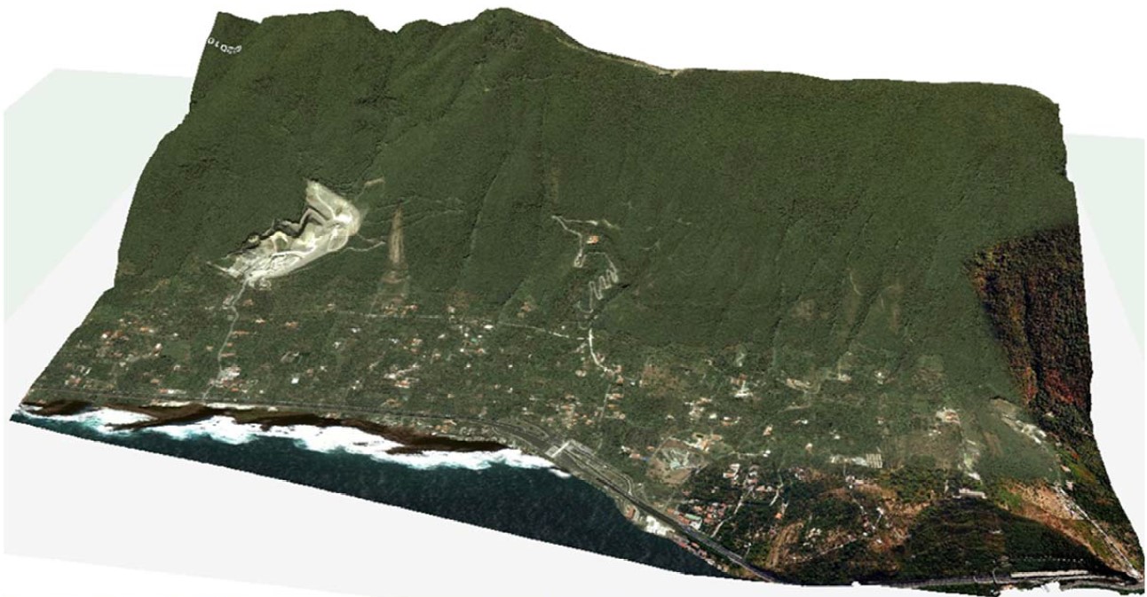
 Data input: To demonstrate its use, SMCE is applied to qualitatively analyse and zone the risk on a hypothetical slope where four hazardous processes were identified: 1) flooding phenomena, 2) hyperconcentrated flows, 3) debris flows and 4) landslides on open slopes. According to the stepwise procedure, as described in the previous section, the parameter maps that characterize the hazard and vulnerability were generated first. The next section describes these input data:    

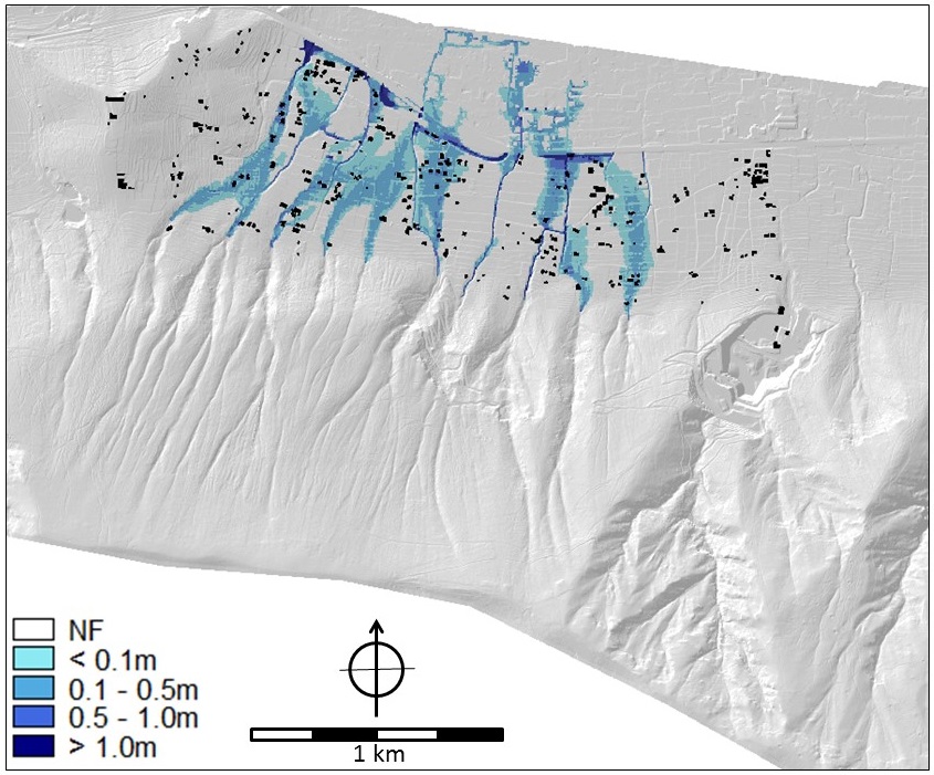
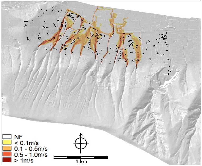
Hazard information: As far as hazard analysis is concerned, the parameter maps of floods, hyperconcentrated flows and debris flows contain depth and velocity values that were the output of modelling analyses (SafeLand Deliverable 2.11 2011, Cascini et al. 2013). In particular, the FLO-2D numerical code (O'Brien et al. 1993) was applied on a high-quality DTM of squared cells of 5m x 5m obtained from a LiDAR survey. The flow parameters were separately evaluated for the ten mountain catchments of the hillslope (Cascini et al. 2013). For the purposes of the participatory process (Scolobig et al. 2013), the hazards were evaluated considering triggering rainfall events with a return period of 20 and 100 years for flooding and 200 years for hyperconcentrated flows and mud (or debris) flows. For the hyperconcentrated flows, three different sets of rheological properties of the soil-water mixtures (in terms of Bingham's yield stress and viscosity) were considered for the analysis. Details on the input data can be found in SafeLand Deliverable 2.11 (2011). For landslides on open slopes, the stability conditions were assessed in terms of safety factors taking into account the soil stratigraphy and using the combined groundwater and slope-stability model (Geoslope 2004a, b). Indiscriminately referring to one of the ten open slopes that are present at the toe of the massif, the average return period of these type of first-time landslides was estimated at once every 20 years; whereas, focusing on a single and well defined  open slope, the return period increases up to 200 years. The run-out distance was evaluated from geomorphologic criteria, taking into account the extent of the debris fans. Some of the parameter maps for all four hazards are shown in Figures 5 to 9.

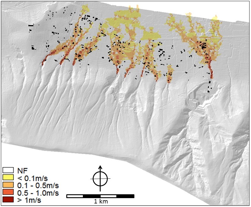 Figure 5. Flood maps for the 20 year flood. LEFT Flow depth (m) and RIGHT flow velocity (m/s). Map names in criteria trees: Flow_depth_020y and flow_velocity_020y. 

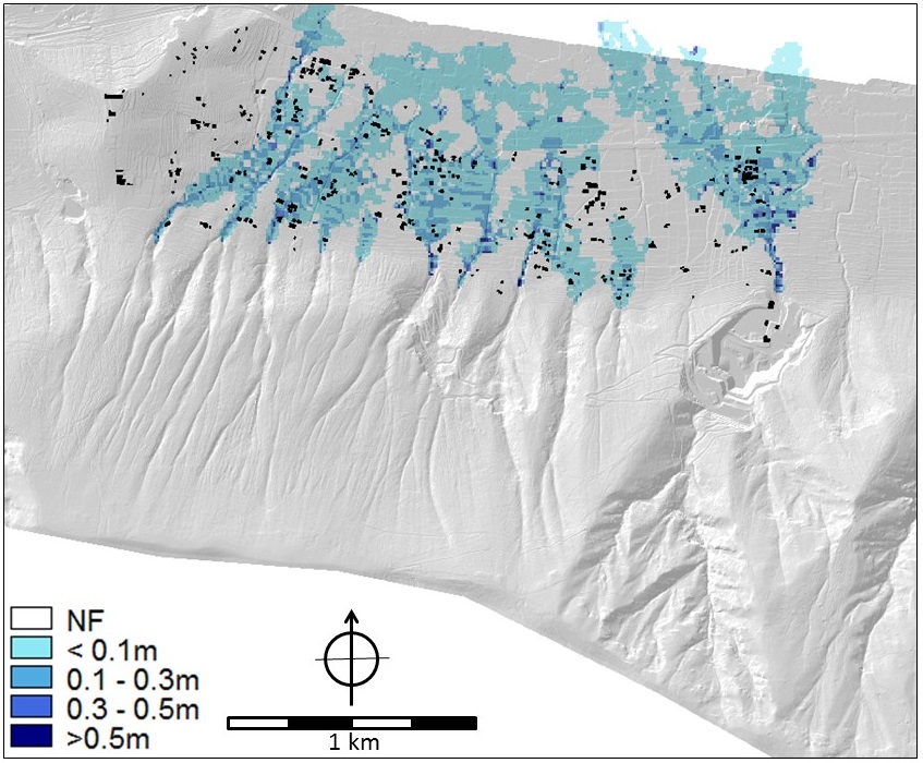
Figure 6. Flood maps for the 100 year flood. LEFT: Flow depth (m) and RIGHT flow velocity (m/s). Map names in criteria tees: Flow_depth_100y and flow_velocity_100y.

 

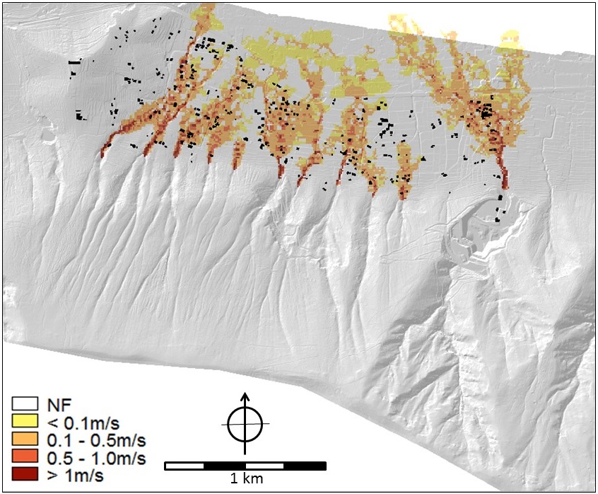Figure 7. Hyperconcentrated Flow - type 1 (least viscous). LEFT: Flow depth (m) RIGHT: Flow velocity (m/s). Mapnames in the criteria trees: HCF_sc1_depth_smce and HCF_sc1_velocity_smce.

 

 

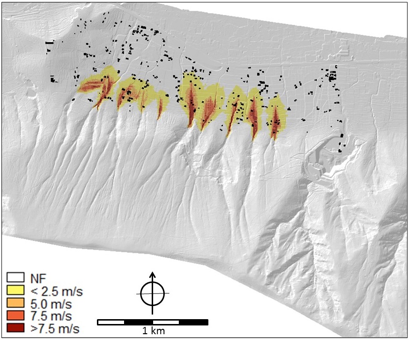
Figure 8. Mud flows. Flow velocity (m/s). Map name in criteria trees: mudflow_velocity_smce.

 

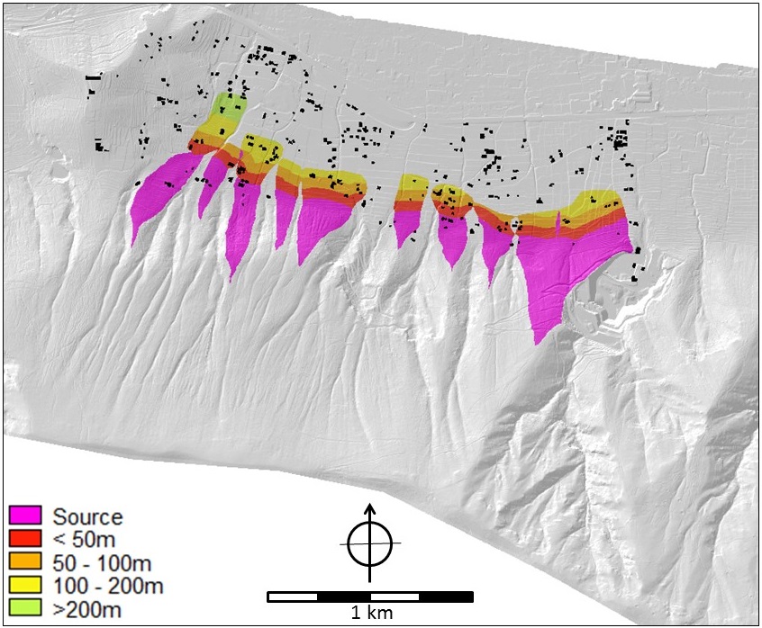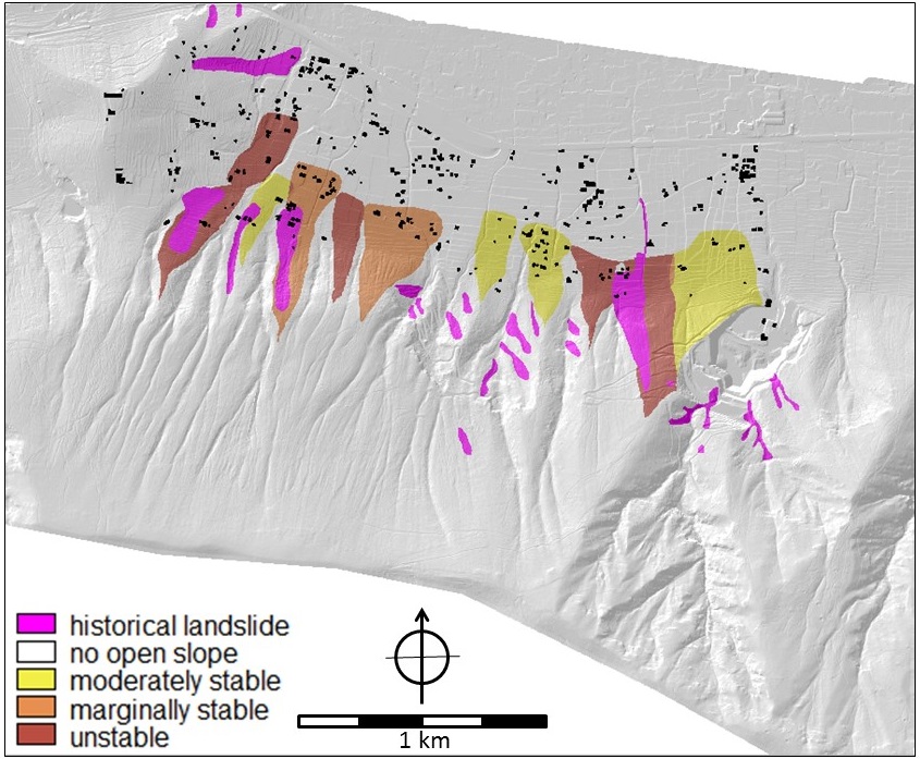
 Figure 9. Landslides and slope stability. LEFT: Stability of the slopes with indication of potential runout, historic landslides are indicated in purple. Map name in criteria trees: open_slope_stability and landslide. RIGHT: potential maximum runout distance (in meters) of landslides originating from the slopes. Map name in the criteria trees: landslide_distance. 

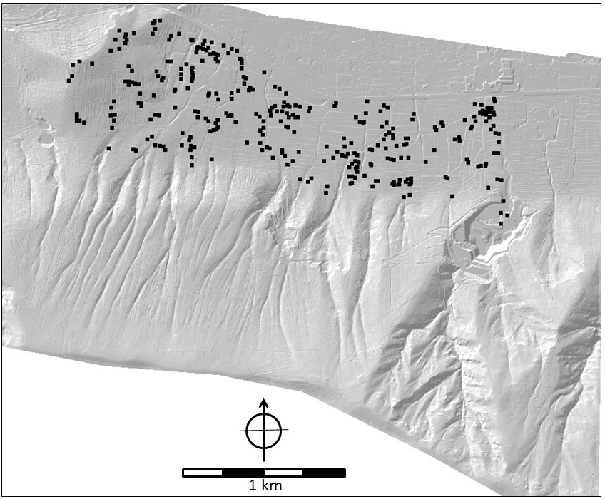
Vulnerability information: Referring to the vulnerability, the necessary information was derived from three source maps: 1) the land use map (Figure 10), 2) the road type map (Figure 11); and 3) the building footprint map (Figure 12). This last map contained additional attribute information for each building, such as number of inhabitants, number of floors, building material and type of occupancy. The building map was also used to calculate the distance-to-buildings map (Figure 13).

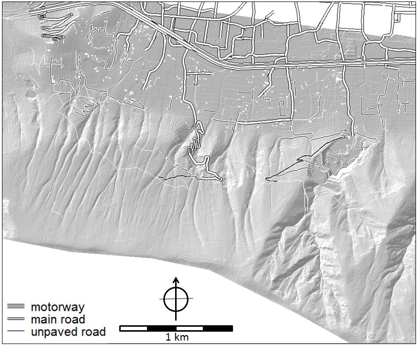 Figure 10 (left). General land use map of the area. Figure 11 (right). Road type map of the area.

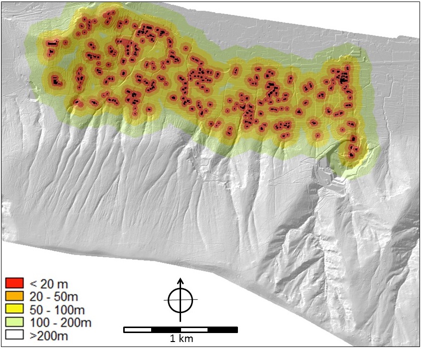Figure 12 (left). Building map. Attribute info: number of floors, building material (wood, brick, reinforced concrete), area (size in m2), use (residential, warehouse, restaurant), and number of inhabitants.

Figure 13 (right). Distance to buildings (in meters). 

Analysis: The decomposition of the problem into a tree-like structure can be done in various ways. Figure 14 shows two structuring approaches. In the first approach all hazard related criteria are grouped in a hazard criteria tree and all vulnerability related criteria are grouped in a vulnerability criteria tree. The resulting generic hazard- and vulnerability maps are then combined into a generic risk map. In the second approach vulnerability is considered as a function of the hazard. For each hazard a hazard specific vulnerability map is defined which results in four hazard-specific risk maps. In a final step, these four maps are then combined into a multi-hazard risk map. In this chapter we will demonstrate approach 1.

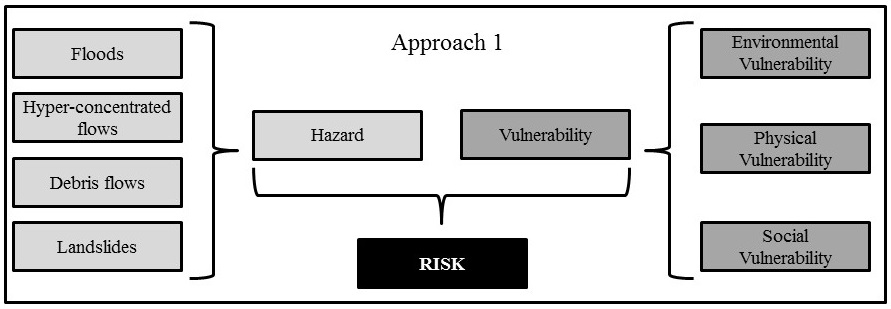
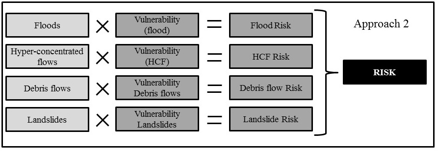
Figure 14. Scheme of the two adopted approaches to SMCE for multi-hazard risk analysis.

 

Generic multi-hazard risk analysis - approach 1

Design of the criteria tree for multi-hazard: Table 1 shows the structuring for the generic multi-hazard analysis. Each hazard is divided into subcategories including hyperconcentrated flows differentiated in terms of rheological properties of the soil-water mixture and flooding phenomena with different return period.  At the lowest level the criteria are defined such as depth and velocity maps. In the right-hand column the corresponding data source (map) is defined. These are the maps that were presented in the previous section.

Criteria that contribute more to the objective receive a higher weight than those that contribute less. Weights were primarily assigned based on the return period T of the hazard, resulting in a five times higher weight for landslides on open slopes (T = 20 years) than the other hazards (T = 200 years) with the exception of flooding phenomena because it was perceived by the stakeholders as a nuisance rather than as a hazard (Scolobig 2013). Therefore, it received a lower weight.

Because the three types of HCF have the same annual probability of occurrence, all three received the same weight. Each flow type was characterized by a combination of maximum velocity and maximum inundation depth. In this example, inundation depth was considered as contributing more to the hazard than flow velocity and therefore received a higher weight (0.75 vs. 0.25). Of course, different work assumptions do not change the structure of the method but only influence the final result.

The 20 year return period flood has a five times higher probability of occurrence than the 100 year flood and therefore received a five times higher weight (0.83 vs. 0.17). The same ratio was applied in estimating the relative contribution to the hazard of depth vs velocity. The difference of this ratio of 5:1 vs. 4:1 in the case of HCF can be explained by the fact that the contribution to the hazard of the velocity in the HCF is considered slightly higher because HCF has a higher density of the flowing mixtures. At the same velocity HCF has a higher momentum than water and is therefore more hazardous and can cause more damage. 

Table 1: Criteria tree for hazard; The right-hand column shows the input indicator maps (not-shaded) and the output "˜composite index' maps or results (shaded). The final outcome - the composite index map or decision - is in this case the map "hazard_current", as defined at the top of the right-hand column. (A: "+" is benefit, "-" is cost; B: "i" is input map, "o" is output map)

 

For mud flows only the maximum flow velocity map was considered as indicator. In this regard, it is worth to mention that - for this kind of phenomenon, characterized by a peculiar kinematics in the propagation stage - consequences related to the impact of the flowing mass to the exposed buildings can be roughly predicted on the basis of the maximum velocity at the impact (Faella and Nigro 2003; Faella 2005).

Three maps were used in analysing the landslide hazard: 1) the slope stability map, 2) the map with historic landslides and 3) the potential maximum run-out map. Most weight was given to the maps that resulted from the deterministic slope stability analysis and runout assessment: 0.60 and 0.30 respectively. A small weight (0.10) was assigned to historic landslides although one can argue that since these slides have occurred, stability has been restored. However, it cannot be excluded that historic events may be the trigger of new, future events. In addition, one can also argue that historic slides may indicate instable conditions in their immediate vicinity.

Where the weighing procedure gives the relative importance of each criterion with respect to the other criteria, the standardization procedure rescales each criterion internally to a scale of 0 to 1. The way this was done is given behind the description of the criteria (Table 1). For different types of maps different methods can be applied. Continuous data (values) can be rescaled using rescaling functions.

The multi-hazard map is shown in Figure 15. This so-called composite index map shows, on a scale from 0 to 1, the areas which are most (1) and least (0) hazardous. In Figure 15 the dominance of landslides on open slopes as most hazardous process is clearly visible in the end result.

 

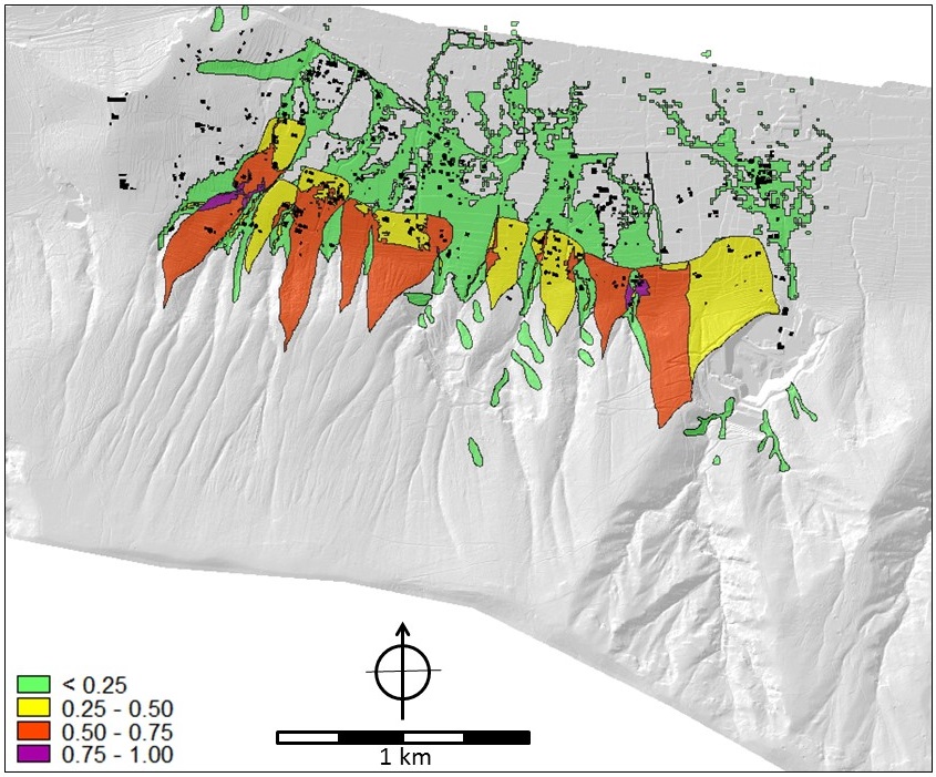
 Figure 15. Composite index map for multi-hazard. A low score indicates least hazardous and a high score most hazardous.

Design of the criteria tree for multi-hazard vulnerability: In this example three different types of vulnerability are considered, namely: environmental, physical and social - see also Methodology Book chapter 5.3.

Environmental vulnerability evaluates the potential impacts of events on the environment (flora, fauna, ecosystems, biodiversity). As a proxy indicator, the land use map was used; it consisted of four units (Fig. 9): 1) urban areas, 2) forest, 3) orchards and small fruits, and 4) unknown. Each of these units was assessed for its environmental quality with using a direct-weight-assignment method. Urban areas received the lowest environmental quality grade (0) and forest the highest (1). The other two units received the intermediate grade of 0.5.

Physical vulnerability is the potential for physical impact on the built environment. According to Fell et al. (2008) it is defined as the degree of loss to a given element-at-risk or set of elements-at-risk resulting from the occurrence of a natural phenomenon of a given intensity, and expressed on a scale from 0 (no damage) to 1 (total damage). The following groups of indicators for analysing the physical vulnerability were used: 1) building vulnerability (based on construction material and number of floors), 2) immediate area surrounding the buildings (< 20 m) for property damage, and 3) the potential for damage (based on land use and building size).

Social vulnerability is the potential impact of events on groups within the society and it considers public awareness of risk, ability of groups to self-cope with catastrophes, and the status of institutional structures designed to help them cope. The social vulnerability was derived from: 1) Roads (based on their importance for immediate rescue services), 2) building occupancy to estimate the amount of people present during day-time, 3) building inhabitants to estimate the amount of people present during night-time, and 4) the number of floors as means for vertical evacuation.

The assignment of the weights to each of the three vulnerability types is highly subjective and is obviously related to the perception of the assessors and their preferences. In this particular case special emphasis was given to the social vulnerability (weight = 0.6) with physical vulnerability on a second place with a weight of 0.35. The environmental vulnerability was given the lowest weight (0.05). The criteria tree is shown in Table 2 and the resulting generic vulnerability map in Figure 16. The highest vulnerability values are associated with the buildings and their immediate surroundings, as well as with the land use type urban area. The road network, as essential lifeline during rescue and civil protection operations, is also clearly distinguishable in the vulnerability map. 

Table 2: Criteria tree for multi-hazard vulnerability. The final outcome - the composite index map, or decision - is in this case the map vulnerability_current, as defined at the top of the right-hand column

.

 

 

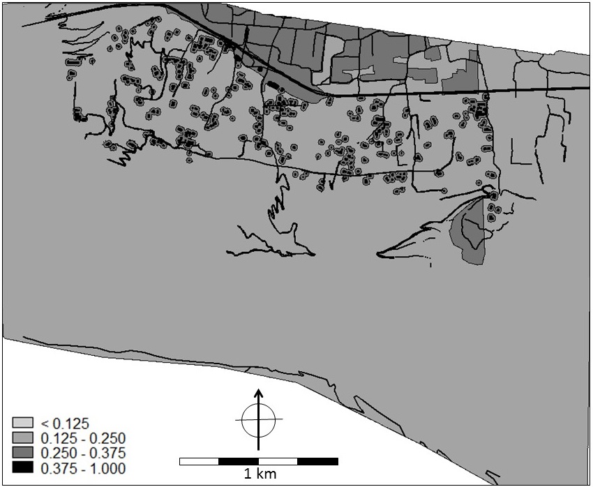
 Figure 16. Composite index map for multi-hazard vulnerability. A low score indicates least vulnerable and a high score most vulnerable. 

The resulting generic multi-hazard risk map: Figure 17 presents the final generic multi-hazard risk map as the product of the hazard and vulnerability maps. This index map - also on scale of minimum 0 and maximum 1, gives an impression of the relative spatial distribution of the risk in the study area.

  

Figure 17. The composite index map for generic multi-hazard risk in case the hazards are weighed according to their expected return periods; high values represent areas of high risk, low values areas of low risk.

 

An example of scenario analysis: the effects of landslide risk mitigation: Suppose active control works are installed to reduce the average frequency of landslide occurrence on open slopes from 1 in 20 years to 1 in 100 years. In the SMCE this is done by adjusting the weights. Figure 18 shows the resulting qualitative risk map and it is clearly visible that the relative risk due to landslides has been reduced with respect to the relative risk of the other hazardous phenomena. SMCE cannot show that the absolute levels of risk have been reduced in the area but it does show the spatial changes in relative. Because landslide risk has been mitigated, the risk due to flow-like phenomena (i.e. hyperconcentrated flows and debris flows) is now more pronounced, in relative terms, than in Figure 17. 

 

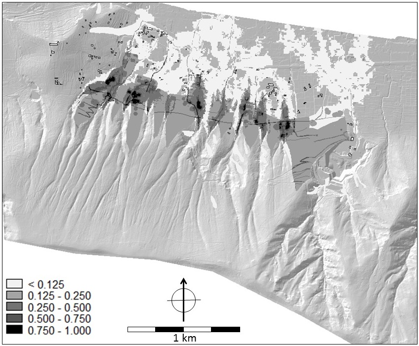
Figure 18. The composite index map for generic multi-hazard risk in case all hazards are equally weighted - i.e. when mitigation works have been put in place to reduce landslide hazard from 1 in 20 years to approximately 1 in 100 years.

Discussion

The composite index maps of the multi-hazard risk in figure 17 show the division of the study area into degrees of relative risk whose scores are ranging from 0 to 1. In this example a high score relates to relatively high risk and that a value close to zero means that the relative risk is low. However, as a general rule, the composite index map values per se do not have meaning. The values are dimensionless and cannot be interpreted outside their context. They only have meaning compared with other values within the map and, provided that standard value functions and weights have been applied to different locations or different alternatives, only relative and not absolute comparisons can be made.

The fact that the composite index map values can only be interpreted in comparison with other values within the map makes it difficult to compare different scenarios in SMCE. For instance, in the present work a scenario with landslide mitigation measures and how that would affect the spatial risk distribution was presented. In these examples it is possible to observe that the new spatial risk distribution differs from the scenario without mitigation measures but it is not possible to see differences in absolute risk values: Both maps (without and with mitigation measures) show the risk index values on a scale from 0 to 1. One would have to go back to the problem structure and the input maps to understand the origin of changes in hazard, vulnerability and risk. 

Based on these observations, the following can be observerd regarding the strengths and weaknesses of the use of SMCE for hazard and risk assessment: 

Strengths

Integration of multiple parameters: SMCE allows the incorporation of multiple parameters (criteria) in defining both hazard and vulnerability. For example, referring to the example, ten criteria were combined to evaluate the multi-dimensional aspect of the vulnerability (including social, physical and environmental factors) - ranging from land use information to building occupancy.

Multi-hazard assessment: In the same manner that SMCE allows the incorporation of multiple parameters for hazard or vulnerability assessment, so does it allow the integration of multiple hazards into an integrated multi-hazard assessment. In the example it was demonstrated how four separate hazards were combined. The estimated return periods of the hazards were used in the assignment of weights to emphasize the dominant hazard.

Intrinsic logic: The SMCE procedure makes the stakeholders (or assessors) apply a certain intrinsic logic which - if followed through in a systematic manner - will result in a logical conclusion. For each criterion, the assessors must decide how it will contribute to the risk: is it a cost or a benefit?. For instance the higher the number of inhabitants in a building is, the higher the vulnerability is;  therefore this number will contribute positively to the risk. For landslide run-out distance the opposite holds. The shorter the distance a house is separated from the foot of the slope, the more likely a landslide may affect it. The further away the less chance a landslide will travel that far. Therefore the less the distance the more it contributes to risk.

Applicability: SMCE does not require a predefined set of data to make the assessment, nor does the dataset need to be complete. SMCE allows the stakeholders to evaluate the hazard, vulnerability and risk with the data that are available. This flexibility increases its applicability.

Inclusiveness: SMCE is not only a tool to calculate a result, but it is also a procedure to facilitate collaborative decision making. It allows multiple stakeholders - also with conflicting views and different perceptions - to go through the process in small steps. The stakeholders can use the procedure of SMCE to reach agreement on the objectives of the risk map, the set of criteria and the processing of this information. If agreement exists at all stages of the SMCE-procedure, they must also agree on the outcome: the risk map. In this way SMCE adds to the decision-making process in the sense that it identifies agreements and disagreements between the stakeholders, that it brings understanding, supports learning-by-doing and that it reveals areas where further information is needed.

Alternatively it is possible to have different stakeholders make individual assessments with different criteria trees and and to evaluate the differences in outcome afterwards. It may be that different assessments (based on different viewpoints, etc) still produce commonalities in the end results. These may form the basis for a compromise solution.

It should be noted that due to the technical GIS environment required for SMCE, the stakeholder process requires support from a GIS expert.

Sensitivity analysis: SMCE can be used for sensitivity analysis to find out how much uncertainty in one of the criteria - or its weights or normalization - affects the outcome. In some cases this may help in the discussion if it shows that a disagreement between stakeholders does not have serious implications for the result. Sensitivity analysis serves to test the robustness of the decision with respect to uncertainties in the parameter maps, weights, value functions and decision rules. 

Weaknesses

Subjectivity: The main characteristic of SMCE is that there are no rules in designing the criteria tree, in the assignment of the weights or in the normalization process. In fact, defining the value functions is one of the major discussion topics in the multi-criteria evaluation procedure. The assessor is most likely to be a group of people (experts, stakeholders). They either form a team or a coalition, but together they have to reach agreement on the value functions for each parameter included in the assessment. This should avoid possible bias from individual members, but raises new problems like composition of the expert group (number and backgrounds of the experts) and the interaction within the group. This can result in discussion and bartering about the value functions which may seem unscientific. However, given scientific uncertainty about complex phenomena of mass movement and flooding it is currently the best that can be achieved.

Replicability: SMCE is a very flexible tool that can be applied in many cases with different datasets. However, this makes comparison between different studies difficult, if not impossible. Another group of stakeholders will probably obtain different results.  

Meaning: The result of SMCE, the decision, is a so-called composite index with values between 0 and 1. In the example of risk assessment for the case study of Nocera Inferiore, a high score means that the conditions at those locations are very suitable for high risk - i.e. high hazard and high vulnerability values. A value close to zero means that the risk is low. However, the composite index map values per se do not have meaning. The values are dimensionless and cannot be interpreted outside their context. They only have meaning compared with other values within the map and provided that standard value functions and weights have been applied to different locations or different alternatives, relative, not absolute comparisons could be made.

Comparability: The fact that the composite index map values can only be interpreted in comparison with other values within the map makes it difficult to compare different scenarios in SMCE. For instance, in the example a scenario with landslide mitigation measures and how that would affect the spatial risk distribution was presented. In that example it was possible to observe that the new spatial risk distribution differs from the scenario without mitigation measures, but it was not possible to see differences in absolute risk values. Both maps show the risk index values on a scale from 0 to 1. 

Conclusions

This chapter set out to demonstrate the use of Spatial Multi-Criteria Evaluation (SMCE) as a qualitative tool for the analysis and zoning of multi-hazard risk. In the example four different hazards were identified, namely: flooding phenomena, hyperconcentrated flows, debris flows and landslides on open slopes. To this aim, multiple parameters (criteria) were incorporated in defining both hazard and vulnerability. For example, referring to the case study at hand, ten criteria to evaluate the multi-dimensional aspect of the vulnerability (including social, physical and environmental factors) - ranging from land use information to building occupancy - were combined. This SMCE quality may allow a wider definition of hazard and vulnerability than in quantitative methods. 

More generally - although there are no rules in designing the criteria tree, in the assignment of the weights or in the normalization process - SMCE procedure forces the involved stakeholders to apply a certain intrinsic logic which, if followed through in a systematic manner, will result in logical and agreed conclusions. This should avoid possible bias from individual members, but raises new problems like composition of the expert group (number and backgrounds of the experts) and the interaction within the group. In any case, it must be stressed that SMCE is not only a tool to calculate a result, but it is also a procedure to facilitate collaborative decision making (e.g. in identifying priority areas for actions to reduce risk) among experts and multiple stakeholders, also with conflicting views and different perceptions. 

SMCE does not require a predefined set of data to make the analysis, nor does the dataset need to be complete. SMCE allows the assessors to evaluate the hazard, vulnerability and risk with the data that are available. This flexibility increases its applicability; however, the stakeholders should be aware of the potential and limitations of the obtained SMCE results with respect to both quality and quantity of the available input data. 

Acknowledgments

The work described in this chapter was supported by the project SafeLand "Living with landslide risk in Europe: Assessment, effects of global change, and risk management strategies" under Grant Agreement No. 226479 in the 7th Framework Programme of the European Commission. This support is gratefully acknowledged. 

References

Ackoff RL (1981) The art and science of mess management. Interfaces 11(1): 20-26.

Alkema D (2007) Simulating floods; on the application of a 2D-flood model for hazard and risk assessment. PhD thesis, University of Utrecht.

Beinat E (1997) Value Functions for Environmental Management, Dordrecht etc., Kluwer.

Boerboom LGJ, Alan ÖO (2012) Implementation, Challenges and Future Directions of Integrating Services from the Gis and Decision Science Domains: A Case of Distributed Spatial Multi-Criteria Evaluation. OSGeo Journal, 10:49-54.

Borrows P (1999) Issues for flood warning in extreme events. Report of RIPARIUS Expert Meeting 1. Centre for Ecology and Hydrology (CEH), Wallingford, UK.

Burrough PA, McDonnell RA (1998) Principles of Geographical Information Systems. Oxford University Press, UK.

Carver SJ (1991) Integrating multi-criteria evaluation with geographical information systems, International Journal of Geographical Information Systems, 5(3); 321-339.

Cascini L, Ferlisi S, De Chiara G (2013) The Quantitative Risk Assessment for hyperconcentrated flows in Nocera Inferiore (southern Italy). This issue

Castellanos Abella EA (2008) Multi - scale landslide risk assessment in Cuba. PhD thesis University of Utrecht

Chen K, Blong R, Jacobson C (2001) MCE-RISK: integrating multicriteria evaluation and GIS for risk decision-making in natural hazards. Environmental modelling and software 16. pp 387-397.

Dang NM, Babel MS Luong HT (2011) Evaluation of flood risk parameters in the Day River flood diversion area, Red River delta, Vietnam. Nat. Hazard (2011) 56:169-194

SafeLand Deliverable 2.11 (2011) QRA case studies at selected "hotspots". Synthesis of critical issues. Edited for the SafeLand European project by Corominas J and Mavrouli O. Available at http://www.safeland-fp7.eu

Densham PJ (1991) Spatial decision support systems, In: D. J. Maguire, M. S. Goodchild and D. W. Rhind (eds) Geographical information systems: principles and applications, London: Longman, pp. 403 - 412.

Faella C (2005) Flowslide effects on costructions. Panel Report. Proceedings of the International Conference on “Fast Slope Movements – Prediction and Prevention for Risk Mitigation” (Picarelli L. ed.), Naples (Italy). Vol. 2, 53-61, Pàtron Editore (Bologna, Italy).

Faella C, Nigro E (2003) Dynamic impact of the debris flows on the constructions during the hydrogeological disaster in Campania-1998: failure mechanical models and evaluation of the impact velocity. Proceedings of the International Conference on “Fast Slope Movements – Prediction and Prevention for Risk Mitigation” (Picarelli L. ed.), Napoli. Vol. 1: 179-186. Pàtron Editore (Bologna, Italy).

Fell R, Corominas J, Bonnard Ch, Cascini L, Leroi E, Savage WZ on behalf of the JTC-1 Joint Technical Committee on Landslides and Engineered Slopes (2008) Guidelines for landslide susceptibility, hazard and risk zoning for land use planning. Engineering Geology, 102(3-4):85-98.

Gendreau N (1998) Protection objectives in flood-risk prevention. Proceedings of the British Hydrological Society International Conference, Exeter, UK 6‑10 July 1998, p. 145‑154.

Geneletti D (2002) Ecological evaluation for environmental impact assessment. PhD thesis. Netherlands Geographical Studies 301.

Geo-Slope (2004a) Slope stability analysis with SLOPE/W, user's guide version 6.02. GEO-SLOPE International Ltd., Calgary, Alberta, Canada.

Geo-Slope (2004b) Groundwater seepage analysis with SEEP/W, user's guide version 6.02. GEO-SLOPE International Ltd., Calgary, Alberta, Canada.

Herwijnen MV (1999) Spatial Decision Support for Environmental Management, Amsterdam, PhD thesis. Free University Amsterdam.

Hungr O, Evans SG, Bovis MJ, Hutchinson JN (2001) A review of the classification of landslides of the flow type. Environmental & Engineering Geoscience, 7(3): 221-238

Hwang CL, Masud ASM (1979) Multi-objective decision-making – methods and applications: a state of the art survey. Springer, Berlin.

Jonkman SN, Vrijling JK, Vrouwenvelder ACWM (2008) Methods for the estimation of loss of life due to floods: a literature review and a proposal for a new method. Natural Hazards 46:353–389

Lorenz CM (1999) Indicators for sustainable river management. PhD‑thesis, Vrije Universiteit Amsterdam, the Netherlands.

Malczewski J (1999) GIS and multi-criteria decision analysis. Wiley and sons, Inc. USA. Pp 392.

Malczewski J (2006) Gis-Based Multicriteria Decision Analysis: A Survey of the Literature. International Journal of Geographical Information Science, 20, 703-726.

Narasimhan H, Ferlisi S, Cascini L, Faber M, De Chiara G. (2013) A cost-benefit analysis of mitigation options for optimal management of risks posed by flow-like mass movement phenomena. This issue

O’Brien JS, Julien PY, Fullerton WT (1993) Two-dimensional water flood and mudflow simulation. Journal of Hydraulic Engineering ASCE, 119(2): 244-261.

Penning‑Rowsell EC, Tunstall SM (1996) Risks and resources: Defining and managing the floodplain. In: Andersen, M.G., Walling, D.E. and Bates, P.D. (Eds) Floodplain resources. John Wiley and Sons, Ltd. London, UK.

Pfeffer K (2003) Integrating spatio-temporal environmental models for planning ski runs. PhD thesis. Netherlands Geographical Studies 311.

Rashed T, Weeks J (2003) Assessing vulnerability to earthquake hazards through spatial multicriteria analysis of urban areas. Int. Journal of Geographical Information Science. Vol 17. No 6, 547-576.

Rothenberg J (1975) Cost-Benefit analysis: A methodological exposition. In (eds) Guttentag, M. and Strüning E.L. Handbook of evaluation research. Sage Publications, USA.

Saaty TL (1980) The analytical hierarchy process: Planning, priority setting and resource allocation. McGraw-Hill, USA.

Scott Morton, MS (1971) Management Decision Systems; Computer-based support for decision-making. Boston, Division of Research, Graduate School of Business Administration, Harvard University.

Scolobig A (2013) Stakeholder perspectives on landslide risk management. This Issue.

Scolobig A, Bayer J, Cascini L, Ferlisi S (2013) A participatory process for landslide risk mitigation: compromise versus consensus. This Issue.

Sharifi, MA. Van den Toorn, Rico, A and Emmanuel, M (2002) Application of GIS and Multicriteria Evaluation in locating sustainable boundary between the Tunari National Park and Cochabamba city (Bolivia). Journal of Multi-Criteria Decision Analysis 11, pp. 151-164.

Sharifi, MA and Retsios, V (2003) Site selection for waste disposal through spatial multiple criteria decision analysis. In: Proceedings of the 3rd International conference on decision support for telecommunications and information society DSTIS, 4-6 September 2003, Warsaw, Poland. 15 p.

Témez, JR (1991) Planificación hidrológica‑ordenación de zones inundables, CEDEX, Madrid, Spain.

Ullman, D G (2006) Making Robust Decisions: Decision Management for Technical, Business, & Service Teams Trafford Publishing.

Zucca, A (2005) Sviluppo sostenibile del territorio: Agenda 21 locale e valutazione ambientale strategica. Proposta di metodologie per la gestione dell’informazione spaziale nei processi decisionali. Unpublished PhD thesis, Università degli studi di Milano-Bicocca.